Chapter 8 Modeling Categorical Time Series
8.1 Introduction
This chapter describes Bayesian dynamic generalized linear models (DGLMs) for categorical time series. Section 8.2 discusses model fitting for a single binomial response time series, while Section 8.3 describes a hierarchical framework for modeling multiple binomial response time series (see Chapter 6 for a discussion on Gaussian hierarchical dynamic models). Modeling time series with more than two categories is discussed in Section 8.4.
The custom functions must first be sourced.
source("functions_custom.R")We use the following packages in this chapter.
library(INLA)
library(tidyverse)
We analyze the following data set.
- Weekly shopping trips
8.2 Binomial response time series
Consider a discrete-valued time series \(Y_t\) whose conditional distribution at time \(t\) is Bin\((m,\pi_t)\), where \(m\) denotes the size of the distribution. Then, \(Y_t\) denotes the number of successes in \(m\) independent Bernoulli trials, and has mean and variance given by \(E(Y_t) = m \pi_t\) and \(\mbox{Var}(Y_t) = m \pi_t (1-\pi_t)\). Following the well known generalized linear modeling approach (McCullagh and Nelder 1989), we can link the mean response \(\pi_t\) to a structured linear Gaussian predictor using a suitable link function. Well known link functions for binomial response modeling include the logit and probit links for \(\pi_t\), given by
\[\begin{align*} \text{logit}(\pi_t) = \log \frac{\pi_t}{1-\pi_t}, \end{align*}\] and
\[\begin{align*} \text{probit}(\pi_t) = \mathcal{N}^{-1}(\pi_t), \end{align*}\] where \(\mathcal{N}^{-1}(.)\) denotes the inverse c.d.f. of the \(N(0,1)\) distribution. Note that we have used \(\mathcal{N}^{-1}\) instead of the usual notation in the literature of \(\Phi^{-1}\) to avoid confusion with the matrix of AR coefficients (see Chapter 12). Excellent references on sampling based Bayesian approaches for fitting DGLMs include Dani Gamerman (1998) and West and Harrison (1997). Also, see Refik Soyer and Sung (2013) for a discussion of binary longitudinal response modeling under a probit link.
8.2.1 Example: Simulated single binomial response series
The observation and state equations of a DGLM for a binomial response time series \(Y_t\) with a logit link are shown below:
\[\begin{align} Y_{t}|\pi_{t} & \sim \text{Binomial}(m, \pi_{t}), \notag \\ \text{logit} (\pi_{t}) &= \alpha +\beta_{t,0},\notag \\ \beta_{t,0} &= \phi \beta_{t-1,0} + w_{t,0}. \tag{8.1} \end{align}\] The model assumes a time-varying intercept \(\beta_{t,0}\) following a latent Gaussian AR(1) model to explain \(\text{logit} (\pi_{t})\), where \(|\phi| < 1\) and the state error \(w_{t,0}\) is N\((0,\sigma^2_w)\). We have also included a fixed level \(\alpha\).
We show the model setup on a simulated time series of length \(n = 1000\), with a burn-in of length \(500\). The size \(m\) of the binomial distribution is denoted by bin.size, and will be passed to inla() through the argument Ntrials.
set.seed(123457)
n <- 1000
burn.in <- 500
n.tot <- n + burn.in
bin.size <- 10
sigma2.w <- 0.05
phi <- 0.8
alpha <- 1.3
yit <- beta.t0 <- pi.t <- eta.t <- vector("double", n.tot)
beta.t0 <-
  arima.sim(list(ar = phi, ma = 0), n = n.tot, sd = sqrt(sigma2.w))
for (i in 1:n.tot) {
  eta.t[i] <- alpha + beta.t0[i]
  pi.t[i] <- exp(eta.t[i]) / (1 + exp(eta.t[i]))
  yit[i] <- rbinom(n = 1, size = bin.size, prob = pi.t[i])
}
yit <- tail(yit, n)
The true precision of the state error \(w_{t,0}\) is \(20\), while the true precision of the state variable \(\beta_{t,0}\) is 7.2, which can be computed using the book’s custom function prec.state.ar1():
prec.state.ar1(state.sigma2 = sigma2.w, phi = phi)We fit the model in (8.1) to the simulated data.
id.beta0 <- 1:n
data.bin <- cbind.data.frame(id.beta0, yit)
prior.bin <- list(
  prec = list(prior = "loggamma", param = c(0.1, 0.1)),
  rho = list(prior = "normal", param = c(0, 0.15))
)
formula.bin <-
  yit ~ 1 + f(id.beta0,
               model = "ar1",
               constr = FALSE,
               hyper = prior.bin)
model.bin <- inla(
  formula.bin,
  family = "binomial",
  Ntrials = bin.size,
  control.family = list(link = "logit"),
  data = data.bin,
  control.predictor = list(compute = TRUE, link = 1),
  control.compute = list(
    dic = TRUE,
    cpo = TRUE,
    waic = TRUE,
    config = TRUE,
    cpo = TRUE
  )
)
# summary(model.bin)
format.inla.out(model.bin$summary.fixed[,c(1,2,4)])
##   name      mean  sd    0.5q
## 1 Intercept 1.228 0.044 1.227
format.inla.out(model.bin$summary.hyperpar[, c(1,2,4)])
##   name                   mean  sd    0.5q
## 1 Precision for id.beta0 8.773 2.019 8.533
## 2 Rho for id.beta0       0.818 0.056 0.825
The posterior means for \(\alpha\), \(\phi\) and \(\sigma^2_w\) are 1.228, 0.818 and 8.773 respectively, suggesting that the true parameters in the simulation are recovered well.
Note that if we incorrectly fit a model with no level \(\alpha\) to this data, then neither the posterior mean of \(\phi\) nor the posterior mean of the precision of the state variable are recovered well. In particular, the posterior mean of \(\phi\) increases to \(0.996\) (i.e., it tends to a limit of 1), possibly in order to accommodate the omitted non-zero level. We illustrate this below. We reiterate what we mentioned in Section 3.3, that it is advisable to include a level \(\alpha\) in the model, expecting it to be estimated close to zero in cases when the true level is zero.
formula.bin.noalpha <-
  yit ~ -1 + f(id.beta0,
               model = "ar1",
               constr = FALSE)
model.bin.noalpha <- inla(
  formula.bin.noalpha,
  family = "binomial",
  Ntrials = bin.size,
  control.family = list(link = "logit"),
  data = data.bin,
  control.predictor = list(compute = TRUE, link = 1),
  control.compute = list(
    dic = TRUE,
    cpo = TRUE,
    waic = TRUE,
    config = TRUE,
    cpo = TRUE
  )
)
format.inla.out(model.bin.noalpha$summary.hyperpar[, c(1,2,4)])
##   name                   mean  sd    0.5q
## 1 Precision for id.beta0 1.144 0.451 1.075
## 2 Rho for id.beta0       0.996 0.002 0.996
8.2.2 Example: Weekly shopping trips for a single household
The dataset trips consists of the number of weekly shopping trips for \(N=548\) households across \(n = 104\) weeks (R. Soyer, Aktekin, and Kim 2016). Here, we present our analysis for a single household, while we discuss a model for all households using a hierarchical model in Section 8.3.2. In this example, we set \(m\) or bin.size to be the maximum number of shopping trips taken by this household over the \(104\) weeks, and assume that the observed weekly shopping trips \(Y_t\) has a Bin\((m,\pi_t)\) distribution.
trips.single.household <-
  read.csv("weekly_shopping_single_household.csv",
           header = TRUE,
           stringsAsFactors = FALSE)
tsline(trips.single.household$n.trips,
        xlab = "week",
        ylab = "shopping trips",
        line.color = "red",
line.size = 0.6) 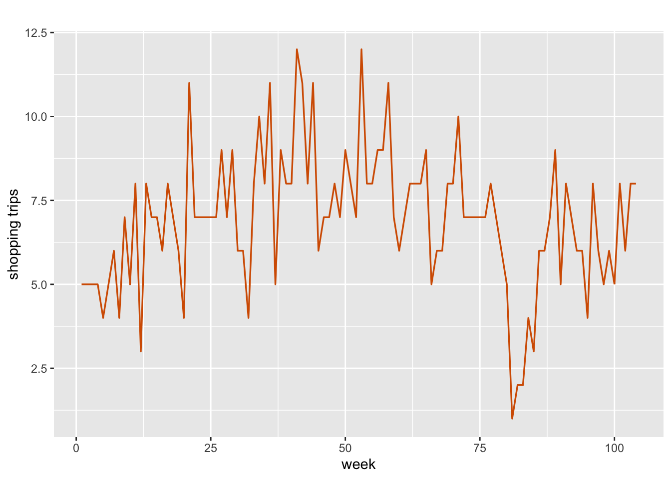
FIGURE 8.1: Number of weekly shopping trips for a single household over n = 104 weeks.
Figure 8.1 shows a plot of \(Y_t\)
for a household with ID 14100859. We divide the data into training and test portions, and create a data frame which includes an index id.beta0.
n <- nrow(trips.single.household)
n.hold <- 6
n.train <- n - n.hold
train.trips.single.household <-
  trips.single.household$n.trips[1:n.train]
test.trips.single.household <-
  tail(trips.single.household$n.trips, n.hold)
bin.size <- max(train.trips.single.household)
id.beta0 <- 1:n
data.single.household <-
  cbind.data.frame(n.trips = c(train.trips.single.household,
                               rep(NA, n.hold)), id.beta0)
To model the time series of trips using (8.1), we use a non-default prior specification for \(1/\sigma^2_w\); specifically, we assume small values of 0.1 and 0.1 for the shape and scale parameters of the log gamma distribution, leading to a diffuse prior. The AR(1) parameter has the default prior for its internal parametrization, as discussed in Chapter 3.
prior.single.household <- list(
  prec = list(prior = "loggamma", param = c(0.1, 0.1)),
  rho = list(prior = "normal", param = c(0, 1))
)
The formula and results are shown below.
formula.single.household <-
  n.trips ~ 1 + f(id.beta0,  model = "ar1", hyper = prior.single.household)
inla.single.household <- inla(
  formula.single.household,
  family = 'binomial',
  Ntrials = bin.size,
  data = data.single.household,
  control.family = list(link = 'logit'),
  control.predictor = list(link = 1, compute = TRUE),
  control.compute = list(
    dic = TRUE,
    cpo = TRUE,
    waic = TRUE,
    config = TRUE
  )
)
# summary(inla.single.household)
format.inla.out(inla.single.household$summary.fixed[, c(1, 3, 5)])
##   name      mean  0.025q 0.975q
## 1 Intercept 0.288 -0.11  0.652
format.inla.out(inla.single.household$summary.hyperpar[, c(1:2)])
##   name                   mean  sd
## 1 Precision for id.beta0 4.625 1.947
## 2 Rho for id.beta0       0.802 0.089
The posterior mean and standard deviation of the hyperparameter \(\phi\) are respectively 0.802 and 0.089, showing that there is a strong positive temporal correlation in the number of shopping trips for this household. We obtain forecasts using inla.posterior.sample(). The contents of each sample can be viewed using inla.single.household$misc$configs$contents.
post.samp <-
  inla.posterior.sample(n = 1000,
                        inla.single.household,
                        seed = 1234)
inla.single.household$misc$configs$contents
## $tag
## [1] "Predictor"   "id.beta0"    "(Intercept)"
##
## $start
## [1]   1 105 209
##
## $length
## [1] 104 104   1
Here “Predictor” returns the predicted \(\eta_t\) for each \(t\). All the elements in tag are stored under latent for each posterior sample. The first \(n\) rows are the “Predictors”, the next \(n\) rows are the posterior estimates of “id.beta0” and the last row contains the posterior estimate of “(Intercept)”. Here, we only show the first and last \(6\) rows of latent for the first sample.
head(post.samp[[1]]$latent)
##             sample:1
## Predictor:1 -0.18534
## Predictor:2 -0.15249
## Predictor:3 -0.20560
## Predictor:4  0.28900
## Predictor:5  0.02523
## Predictor:6 -0.39242
tail(post.samp[[1]]$latent)
##               sample:1
## id.beta0:100    0.1207
## id.beta0:101    0.7823
## id.beta0:102    0.8362
## id.beta0:103    0.6775
## id.beta0:104    0.1225
## (Intercept):1   0.2945
We transform the predicted \(\eta_{j,t}\) into the predicted \(\tilde{\pi}_{j,t}\) via
\[\begin{align*}
\tilde{\pi}_{j,t} = \frac{\exp(\eta_{j,t})}{1+ \exp(\eta_{j,t})},
\end{align*}\]
for each Monte Carlo realization \(j=1,\ldots,1000\). For each \(j\), we use rbinom() to simulate a fitted response from
Bin\((m,\tilde{\pi}_{j,t})\)
for \(t=1,\ldots,n\), yielding \(1000\) binomial time series. We can then obtain summaries such as the mean, standard deviation, and percentiles from these posterior predictive distributions, as shown below.
fit.post.samp <- vector("list", 1000)
for (j in 1:1000) {
  eta <- post.samp[[j]]$latent[1:n]
  p <- exp(eta) / (1 + exp(eta))
  fit.post.samp[[j]] <- rbinom(n, bin.size, p)
}
fore.mean <- bind_cols(fit.post.samp) %>%
  apply(1, mean)
fore.sd <- bind_cols(fit.post.samp) %>%
  apply(1, sd) %>%
  round(3)
fore.quant <- bind_cols(fit.post.samp) %>%
  apply(1, function(x)
    quantile(x, probs = c(0.025, 0.975)))
obs.fit.single.household <-
  cbind.data.frame(
    observed = trips.single.household$n.trips,
    fore.mean,
    fore.sd,
    quant0.025 = fore.quant[1,],
    quant0.975 = fore.quant[2,]
  )
Figure 8.2 shows the observed weekly shopping trips along with the mean of the forecast values generated from inla.posterior.sample().
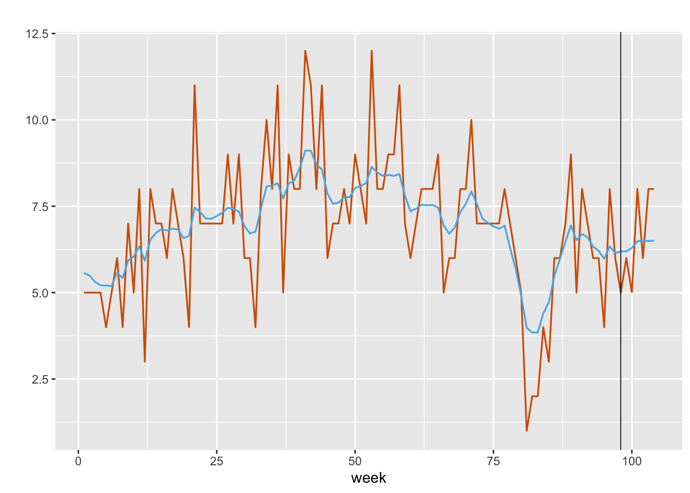
FIGURE 8.2: Observed (red) versus fitted values (blue) for weekly shopping trips of a single household. The black vertical line splits the data into training and test portions.
For this household, the fixed level \(\alpha\) is not significant, and fitting the model without a level \(\alpha\) yields results that are quite similar to what we have shown, as we see below.
formula.single.household.noalpha <-
  n.trips ~ -1 + f(id.beta0,  model = "ar1", hyper = prior.single.household)
inla.single.household.noalpha <- inla(
  formula.single.household.noalpha,
  family = 'binomial',
  Ntrials = bin.size,
  data = data.single.household,
  control.family = list(link = 'logit'),
  control.predictor = list(link = 1, compute = TRUE),
  control.compute = list(dic = TRUE, cpo = TRUE, waic =
                           TRUE)
)
format.inla.out(inla.single.household.noalpha$summary.hyperpar[, c(1:2)])
##   name                   mean  sd
## 1 Precision for id.beta0 3.947 1.571
## 2 Rho for id.beta0       0.844 0.066
8.3 Modeling multiple binomial response time series
In many situations, we may wish to model several binomial response time series \(Y_{it}\) for \(t=1,\ldots,n\) weeks and \(i=1,\ldots,g\) households by aggregating information from all the series. Assume that \(Y_{it}\) follows a Binomial\((m_i, \pi_{it})\) distribution with mean \(E(Y_{it}) = m_i \pi_{it}\) and variance \(\mbox{Var}(Y_{it}) = m_i \pi_{it} (1-\pi_{it})\). Again, each \(\pi_{it}\) is linked to a structured predictor which may be a function of exogenous predictors, or suitable functions of time, or both. In a dynamic model, the state variables may be indexed by \(i\), or \(t\), or both. The coefficients corresponding to the exogenous predictors may be static or dynamic. They can also be constant across \(i\) or vary by \(i\). A similar approach was described in Chapter 6, where we discussed hierarchical DLMs for \(g\) continuous-valued response time series.
8.3.1 Example: Dynamic aggregated model for multiple binomial response time series
Consider the observation and state equations for a hierarchical DGLM (HDGLM) for \(g\) binomial response series under a logit link:
\[\begin{align} Y_{it}|\pi_{it} & \sim \text{Bin}(m_i, \pi_{it}), \notag \\ \text{logit} (\pi_{it}) &= \alpha +\beta_{it,0}+ \beta_{it,1}Z_{it,1}+\beta_{2}Z_{it,2},\notag \\ \beta_{it,0} &= \phi_0 \beta_{i,t-1,0} + w_{it,0}, \notag \\ \beta_{it,1} &= \phi_1 \beta_{i,t-1,1} + w_{it,1}. \tag{8.2} \end{align}\] Here, \(\alpha\) is a fixed level, while the intercept \(\beta_{it,0}\) varies over both \(t\) and \(i\); \(\beta_{it,1}\) is a random effect corresponding to an exogenous predictor \(Z_{it,1}\), and we assume that it varies over both \(t\) and \(i\); and \(\beta_2\) is a static (fixed) effect corresponding to another exogenous predictor \(Z_{it,2}\). Specifically, \(\beta_{it,0}\) follows a latent Gaussian AR(1) process with the same coefficient \(\phi_0\) across all \(i\), where \(|\phi_0| < 1\), and state error \(w_{it,0}\) which is N\((0,\sigma^2_{w0})\). Likewise, \(\beta_{it,1}\) is a latent Gaussian AR(1) process with coefficient \(\phi_1\) (with \(|\phi_1| < 1\)), and state error \(w_{it,1} \sim\) N\((0,\sigma^2_{w1})\).
Values of the sizes \(m_i,~i=1,\ldots, g\), are randomly selected from the set of integers \(\{1,2,\ldots, 12\}\), and the true parameter values are shown below.
set.seed(123457)
g <- 300
n <- 100
burn.in <- 100
n.tot <- n + burn.in
bin.size <- sample(1:12, size = g, replace = TRUE)
alpha <- 1.3
beta.2 <- 2.0
sigma2.w0 <- 0.15
sigma2.w1 <- 0.05
phi.0 <- 0.8
phi.1 <- 0.4
We simulate \(g=300\) binomial response time series from (8.2), each of length \(n=100\) as follows.
yit.all <- z1.all <- z2.all <- vector("list", g)
for (j in 1:g) {
  z1 <- rnorm(n.tot, 0, 1)
  z2 <- rnorm(n.tot, 0, 1)
  yit <-
    beta.0t <- beta.1t <- pi.t <- eta.t <- vector("double", n.tot)
  beta.0t <-
    arima.sim(list(ar = phi.0, ma = 0),
              n = n.tot,
              sd = sqrt(sigma2.w0))
  beta.1t <-
    arima.sim(list(ar = phi.1, ma = 0),
              n = n.tot,
              sd = sqrt(sigma2.w1))
  for (i in 1:n.tot) {
    eta.t[i] <- alpha + beta.0t[i] + beta.1t[i] * z1[i] + beta.2 * z2[i]
    pi.t[i] <- exp(eta.t[i]) / (1 + exp(eta.t[i]))
    yit[i] <- rbinom(n = 1,
                     size = bin.size[j],
                     prob = pi.t[i])
  }
  yit.all[[j]] <- tail(yit, n)
  z1.all[[j]] <- tail(z1, n)
  z2.all[[j]] <- tail(z2, n)
}
yit.all <- unlist(yit.all)
z1.all <- unlist(z1.all)
z2.all <- unlist(z2.all)
Recall from Chapter 6, that to set up a hierarchical model, it is necessary to define appropriate indexes like id.beta0 and id.beta1 to capture the time varying effect and re.beta0 and re.beta1 to allow the intercept and covariate \(Z_{it,1}\) to vary over groups \(i=1,\ldots,g\). In the binomial response models, note that the size Ntrials must be provided for each \(i\) via
bin.size.all <- rep(bin.size, each = n).
id.beta0 <- id.beta1 <- rep(1:n, g)
re.beta0 <- re.beta1 <- rep(1:g, each = n)
bin.size.all <- rep(bin.size, each = n)
data.simul.hbin <-
  cbind.data.frame(id.beta0,
                   id.beta1,
                   yit.all,
                   z1.all,
                   re.beta0,
                   re.beta1,
                   bin.size.all)
We use non-default priors for \(\phi\) and \(\sigma^2_w\) (in their internal parametrizations).
prior.hbin <- list(
  prec = list(prior = "loggamma", param = c(0.1, 0.1)),
  rho = list(prior = "normal", param = c(0, 0.15))
)
The formula and inla() call are shown below, followed by results from fitting the model in (8.2) to this data. The fitted model for the aggregated binomial responses recovers the true parameters well, as seen from the posterior summaries of the fixed effects and the hyperparameters.
formula.simul.hbin <-
  yit.all ~ 1 + z2.all +
  f(id.beta0,
    model = "ar1",
    replicate = re.beta0,
    hyper = prior.hbin) +
  f(
    id.beta1,
    z1.all,
    model = "ar1",
    replicate = re.beta1,
    hyper = prior.hbin
  )
model.simul.hbin <- inla(
formula.simul.hbin,
family = "binomial",
Ntrials = bin.size.all,
control.family = list(link = "logit"),
data = data.simul.hbin,
control.predictor = list(compute = TRUE, link = 1),
control.compute = list(
dic = TRUE,
cpo = TRUE,
waic = TRUE,
config = TRUE,
cpo = TRUE
)
)format.inla.out(summary.simul.hbin$fixed[, c(1:5)])
## name mean sd 0.025q 0.5q 0.975q
## 1 Intercept 1.279 0.014 1.252 1.279 1.306
## 2 z2.all 1.978 0.011 1.956 1.978 2.000
format.inla.out(summary.simul.hbin$hyperpar[, c(1:2)])
## name mean sd
## 1 Precision for id.beta0 2.600 0.098
## 2 Rho for id.beta0 0.811 0.009
## 3 Precision for id.beta1 20.046 3.357
## 4 Rho for id.beta1 0.263 0.3248.3.2 Example: Weekly shopping trips for multiple households
We model the number of weekly shopping trips, i.e., n.trips, of \(g=548\) households over \(n=104\) weeks (R. Soyer, Aktekin, and Kim 2016). We fit a hierarchical model to the binomial responses \(Y_{it}\). The size \(m_i\) of the binomial distribution for each household is taken to be the maximum of the shopping trips across all weeks for that household. The model has a random household-specific and time-varying intercept, but no exogenous predictors.
\[\begin{align} Y_{it}|\pi_{it} & \sim \text{Bin}(m_i,\pi_{it}), \notag \\ \text{logit} (\pi_{it}) &= \alpha+\beta_{it,0} ,\notag \\ \beta_{it,0} &= \phi_0 \beta_{i,t-1,0} + w_{it,0}, \tag{8.3} \end{align}\]
trips <-
  read.csv("Weekly_Shopping_Trips.csv",
           header = TRUE,
           stringsAsFactors = FALSE)
Each row of the data set trips contains the weekly number of trips for each of \(g=548\) households over \(n=104\) weeks. We first convert data from wide data format to long data format, which facilitates our model setup.
g <- nrow(trips)
trips.long <- trips %>%
  pivot_longer(cols = W614:W717, names_to = "week") %>%
  rename(n.trips = value)
n <- n_distinct(trips.long$week)
n.hold <- 6
n.train <- n - n.hold
trips.house <- trips.long %>%
  group_split(panelist)
train.df <- trips.house %>%
  lapply(function(x)
    x[1:n.train, ]) %>%
  bind_rows()
test.df <- trips.house %>%
  lapply(function(x)
    tail(x, n.hold)) %>%
  bind_rows()
We set up indexes and replicates for fitting (8.3).
bin.size <- train.df %>%
  group_split(panelist) %>%
  sapply(function(x)
    max(x$n.trips))
trips.allh <- trips.house %>%
  lapply(function(x)
    mutate(x, n.trips = replace(
      n.trips, list = (n.train + 1):n, values = NA
    )))
id.b0 <- id.house <- rep(1:n, g)
re <- re.house <- rep(1:g, each = n)
trips.allh <-
  cbind.data.frame(bind_rows(trips.allh), id.b0, re, id.house, re.house)
prior.hbin = list(
  prec = list(prior = "loggamma", param = c(0.1, 0.1)),
  rho = list(prior = "normal", param = c(0, 0.15))
)
bin.size.all <- rep(bin.size, each = n)
The formula and results are shown below.
formula.allh <- n.trips ~ 1 +
  f(id.b0,
    model = "ar1",
    replicate = re,hyper = prior.hbin) +
  f(id.house, model = "iid", replicate = re.house)
model.allh <- inla(
  formula.allh,
  family = "binomial",
  Ntrials = bin.size.all,
  control.family = list(link="logit"),
  data = trips.allh,
  control.predictor = list(compute = TRUE, link = 1),
  control.compute = list(
    dic = TRUE,
    cpo = TRUE,
    waic = TRUE,
    config = TRUE,
    cpo = TRUE)
)
# summary(model.allh) format.inla.out(model.allh$summary.fixed[,c(1:2)])
## name mean sd
## 1 Intercept -0.737 0.019
format.inla.out(model.allh$summary.hyperpar[,c(1:2)])
## name mean sd
## 1 Precision for id.b0 2.575 0.104
## 2 Rho for id.b0 0.975 0.002
## 3 Precision for id.house 11.480 1.095Similar to Section 8.2.2, we obtain the posterior predictions and their summaries for all \(g\) households using inla.posterior.sample().
set.seed(1234579)
post.samp <- inla.posterior.sample(n = 1000, model.allh)
model.allh$misc$configs$contents
fit.post.samp <- vector("list", 1000)
fit.house <-
  matrix(0,
         nrow = n,
         ncol = g,
         dimnames = list(NULL, paste("H", 1:g, sep = ".")))
for (j in 1:1000) {
  p <- post.samp[[j]]$latent[1:(n * g)] %>%
    matrix(nrow = n,
           ncol = g,
           byrow = F)
  for (i in 1:g) {
    fit.house[, i] <-
      sapply(p[, i], function(x)
        rbinom(1, bin.size[g], exp(x) / (1 + exp(x))))
  }
  fit.post.samp[[j]] <- fit.house
}
fit.post.samp.all <- fit.post.samp %>%
  lapply(as_tibble) %>%
  bind_rows()
fit.per.house <- vector("list", g)
length(fit.per.house)
str(fit.post.samp.all[, 1])
for (k in 1:g) {
  fit.per.house[[k]] <-
    matrix(c(fit.post.samp.all[[k]]), nrow = n, ncol = 1000)
}
In Figure 8.3, we show plots of observed and fitted values from the hierarchical model (8.3) for a random sample of four households.
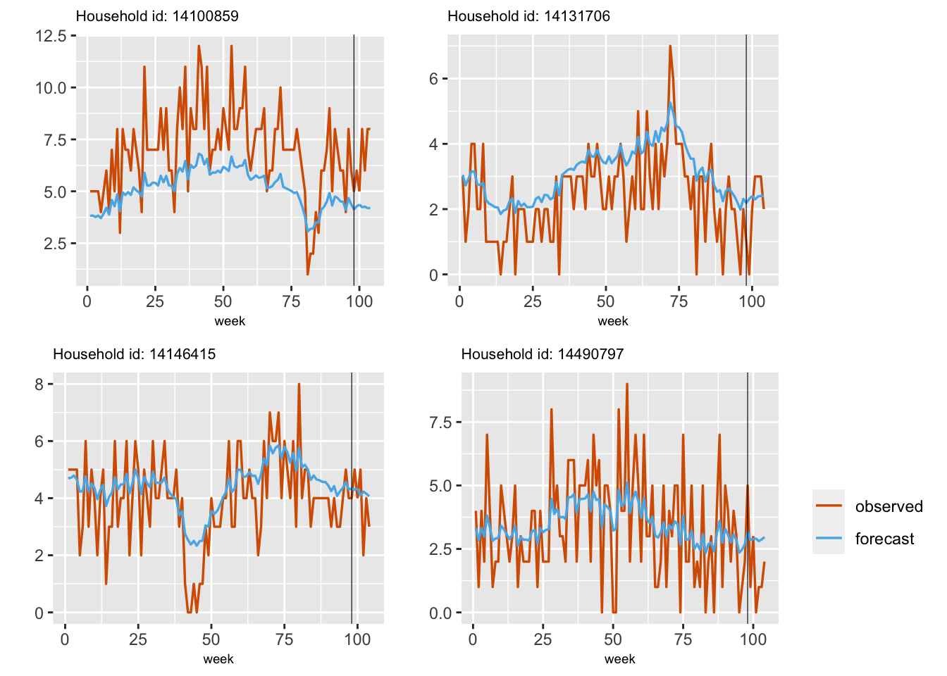
FIGURE 8.3: Plots of observed (red) and fitted (blue) series for four different households.
8.4 Multinomial time series
We end this chapter with a discussion on using R-INLA for modeling categorical time series that follow a multinomial distribution; see Cargnoni, Müller, and West (1997).
Consider a categorical variable with \(J\) mutually exclusive levels. For example, the variable could be the channel for selling a product, with \(J=3\) levels corresponding to brick-and-mortar stores, discount stores, and online sites.
Suppose that out of a total of \(Y_{t+}\) units at time \(t\),
\(Y_{j,t}\) units correspond to level \(j,~j=1,\ldots,J\), such that
\(Y_{j,t}\) are non-negative integers, and \(\sum_{j=1}^J Y_{j,t}=Y_{t+}\).
At each time \(t\), given
\(Y_{t+}\) (i.e., assuming that \(Y_{t+}\) is a fixed constant), suppose that the random vector
\(\boldsymbol{y}_t =(Y_{1,t}, \ldots, Y_{J,t})'\) has a multinomial distribution, \(MN(Y_{t+},\pi_{1,t},\ldots, \pi_{J,t})\), with p.m.f.
\[\begin{align} p(\boldsymbol{y}_t; \boldsymbol{\pi}_t, Y_{t+}) & = \frac{Y_{t+}!}{\prod_{j=1}^J y_{j,t}!} \prod_{j=1}^J \pi_{j,t}^{Y_{j,t}} \notag \\ &= \frac{\Gamma(Y_{t+}+1)}{\prod_{j=1}^J \Gamma(Y_{j,t}+1)} \prod_{j=1}^J \pi_{j,t}^{Y_{j,t}}, \tag{8.4} \end{align}\] where \(\boldsymbol{\pi}_t = (\pi_{1,t},\ldots, \pi_{J,t})'\), \(0 \le \pi_{j,t} \le 1\) and \(\sum_{j=1}^J \pi_{j,t}=1\).
At each time \(t\), assume that we have a \(k\)-dimensional vector of predictors \(\boldsymbol{Z}_{j,t}\), which may also vary by level \(j\). Let \(\boldsymbol{Y}^n = (\boldsymbol{y}_{1}',\ldots,\boldsymbol{y}_{n}')'\) denote the observed multinomial data over \(n\) time periods (i.e., \(t=1,\ldots,n\)). Assume that the proportions \(\pi_{j,t}\) are proportional to the regression function \(g_{j,t}(\boldsymbol{\beta},\boldsymbol{Z}_{j,t}),~j=1,\ldots,J\), where \(\boldsymbol{\beta}\) represents the \(k\)-dimensional vector of regression coefficients. Let \(\eta_{j,t} = \boldsymbol{Z}'_{j,t} \boldsymbol{\beta}\). For simplicity of notation, denote \(g_{j,t}(\boldsymbol{\beta},\boldsymbol{Z}_{j,t})\) by \(g_{j,t}(\boldsymbol{\beta})\), and let \(G_t(\boldsymbol{\beta}) = \sum_{j=1}^J g_{j,t}(\boldsymbol{\beta})\). The most commonly used link function specifies
\[\begin{align} g_{j,t}(\boldsymbol{\beta}) = \exp(\eta_{j,t}) = \exp(\boldsymbol{z}'_{j,t} \boldsymbol{\beta}). \end{align}\]
The multinomial proportions are expressed as functions of \(\boldsymbol{\beta}\), i.e.,
\[\begin{align} \pi_{j,t}(\boldsymbol{\beta}) = \frac{g_{j,t}(\boldsymbol{\beta})}{G_t (\boldsymbol{\beta})}, \tag{8.5} \end{align}\] and the multinomial likelihood can be written as
\[\begin{align} L_{\mathcal{M}}(\boldsymbol{\beta};\boldsymbol{Y}^n) \propto \prod_{t=1}^n \prod_{j=1}^J \left[\frac{g_{j,t}(\boldsymbol\beta)}{G_t(\boldsymbol\beta)}\right]^{y_{j,t}}, \tag{8.6} \end{align}\] where the subscript \(\mathcal{M}\) stands for multinomial. To carry out Bayesian inference, we employ appropriate priors on \(\boldsymbol{\beta}\) and obtain posterior summaries.
Templates for directly specifiying the formulas for Bayesian modeling of categorical data are not currently available in INLA. Instead, INLA uses the well-known
Multinomial-Poisson (M-P) transform to rewrite the multinomial likelihood
in (8.6) as an (see Baker (1994) and Guimaraes (2004)), an approach referred to in the literature as the Poisson-trick (Lee, Green, and Ryan (2017) and Chen and Liu (1997)).
Let \(\phi_t\) be an auxiliary parameter for each time \(t\), and let \(\boldsymbol{\phi} = (\phi_1,\ldots,\phi_n)'\). The idea behind the Multinomial-Poisson (M-P) transformation is to assume that independently for all \(t\), \(Y_{t+}\) is a random variable with
\[\begin{align} Y_{t+} \sim {\rm Poisson}(\phi_t G_t(\boldsymbol{\beta})), \tag{8.7} \end{align}\] and to show that estimating \(\boldsymbol{\beta}\) by maximizing (8.6) is equivalent to estimating it by maximizing
\[\begin{align} L_{\mathcal{P}}(\boldsymbol{\phi},\boldsymbol{\beta}; \boldsymbol{Y}^n) \propto \prod_{t=1}^n \prod_{j=1}^J [g_{j,t}(\boldsymbol{\beta}) e^{\phi_t}]^{y_{j,t}} \exp [- g_{j,t}(\boldsymbol{\beta}) e^{\phi_t}]. \tag{8.8} \end{align}\] See Chapter 8 – Appendix for details.
8.4.1 Example: Simulated categorical time series
Consider a dynamic model for \(\boldsymbol{y}_t = (Y_{1,t}, \ldots, Y_{J,t})'\) with
\[\begin{align} g_{j,t}(\boldsymbol{\beta}_t,\boldsymbol{Z}_{j,t}) &= \exp(\boldsymbol{Z}'_{j,t}\boldsymbol{\beta}_t) = \exp(\eta_{j,t}), {\rm where} \notag \\ \eta_{j,t} & = \begin{cases} \beta_{j,t,0} + \beta C_{j,t} + \delta_j U_{j,t} & \mbox{ if } j=i, \\ \beta C_{j,t} + \delta_j U_{j,t} & \mbox{ if } j \neq i, \end{cases} \tag{8.9} \end{align}\] where the time-varying intercept \(\beta_{j,t,0}\) for the selected category evolves as a random walk
\[\begin{align} \beta_{j,t,0} = \beta_{j,t-1,0} + w_{j,t}, \tag{8.10} \end{align}\] with \(w_{j,t} \sim N(0, \sigma^2_{w_j})\). For instance, if we let \(j=1\), then \(\eta_{1,t}\) for the first category includes a dynamic intercept \(\beta_{1,t,0}\), while the others do not. In (8.9), \(C_{j,t}\) is a category specific predictor over time with a coefficient \(\beta\) which is constant across \(t\) and \(j\), \(U_{j,t}\) is another category specific predictor over time with a category-specific coefficient \(\delta_j\). For more on this setup, see.6
Model D1: Dynamic intercept in a single category
We generate a single categorical time series of length \(n=500\), with \(J=3\) categories, so that, at each time \(t\), \(N=100\) units are categorized into these three groups. Here, \(N\) denotes the multinomial size and \(Y_{j,t}\) denotes the multinomial counts for \(j=1,\ldots,J\) categories at time \(t\). We set up the true parameter values for the model in (8.9) and (8.10), and generate a latent time-varying random effect \(\beta_{1,t,0}\) for the first category.
beta <-  -0.3  # coefficient for C[j,t]
deltas <-  c(1, 4, 3) # category specific coefficients for U[j,t]
param <-  c(beta, deltas)
n <-  1000
set.seed(123457)
# category specific predictor with constant coefficient beta
C.1 <-  rnorm(n, mean = 30, sd = 2.5)
C.2 <- rnorm(n, mean = 35, sd = 3.5)
C.3 <- rnorm(n, mean = 40, sd = 1)
# category specific predictor with category-specific coefficient delta_j
U.1 <- rnorm(n, mean = 2, sd = 0.5)
U.2 <- rnorm(n, mean = 2, sd = 0.5)
U.3 <- rnorm(n, mean = 2, sd = 0.5)
We set up the following function to simulate the time series from model (8.9) and (8.10). Note that we can include a random walk effect for either of the other categories \(j=2\) as \(\beta_{2,t,0}\) or for \(j=3\) as \(\beta_{3,t,0}\) instead of category \(j=1\), by modifying the code below, i.e., uncommenting
random.int[t] for the category we wish to modify and commenting it out from the others.
Multinom.sample.rand <- function(N, random.int) {
  Y <- matrix(NA, ncol = 3, nrow = n)
  for (t in 1:n) {
    eta.1 <- beta * C.1[t] + deltas[1] * U.1[t] +
      random.int[t]
    eta.2 <- beta * C.2[t] + deltas[2] * U.2[t]
    #   + random.int[t]
    eta.3 <- beta * C.3[t] + deltas[3] * U.3[t]
    #   + random.int[t]
    probs <- c(eta.1, eta.2, eta.3)
    probs <- exp(probs) / sum(exp(probs))
    samp <- rmultinom(1, N, prob = probs)
    Y[t,] <- as.vector(samp)
  }
  colnames(Y) <- c("Y.1", "Y.2", "Y.3")
  return(Y)
}
We generate \(\beta_{1,t,0}\) from a random walk with standard deviation 0.1.
rw1.int <- rep(NA, n)
rw1.int[1] <- 0
for (t in 2:n) {
  rw1.int[t] <- rnorm(1, mean = rw1.int[t - 1], sd = 0.1)
}
We then generate the multinomial time series Y.rw1 with size \(N=100\) at each time \(t\), and plot the series, see Figure 8.4.
N <- 100
Y.rw1 <- Multinom.sample.rand(N, rw1.int)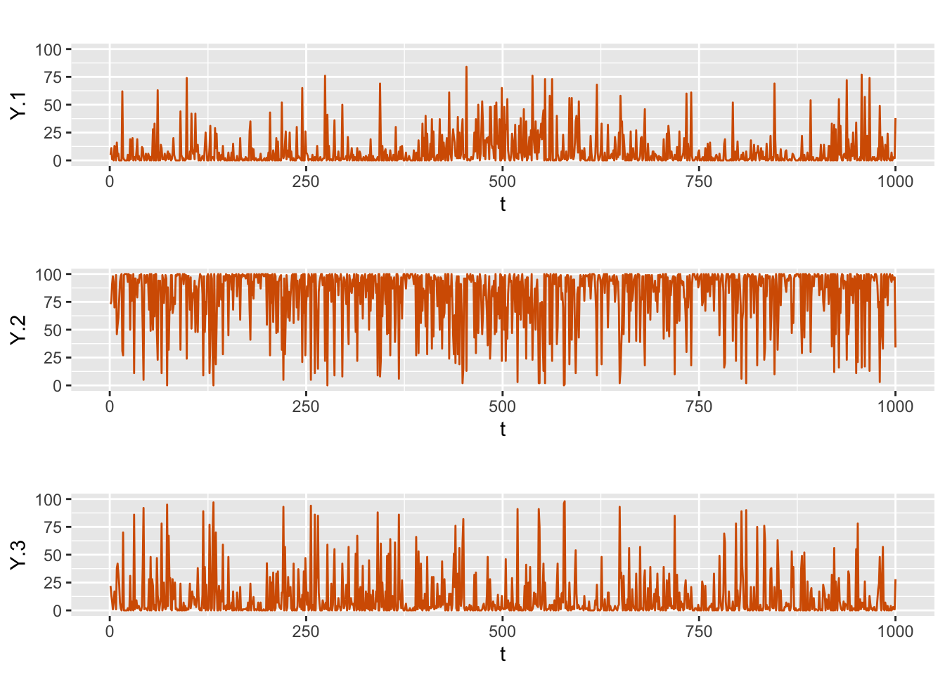
FIGURE 8.4: Simulated multinomial time series from Model D1.
Next, we build the data set to input into R-INLA. This data set will have \(3n\) rows, one for each choice category in each choice situation, Y.1, Y.2, Y.3.
For the predictor \(C_{j,t}\), we use the long format, so we stack C.1, C.2, C.3 into a long vector C in a single column.
For the predictors \(U_{j,t}\), we use three columns, U.1, U.2, U.3, one for each category with \(3n\) rows each. Each column will have the value of the predictor for the corresponding category, and zeros for the other categories.
The data frame additionally includes one more column, i.e., an index column representing the choice situation, with an additional parameter \(\phi\), corresponding to the \(\phi_t\) we included in the M-P transformation. Note that \(\phi_t\) indexes time but remains the same across categories for each time. The following function takes as input a data frame in wide format and transforms it into the structure described above, and sets up the index for the dynamic intercept \(\beta_{1,t,0}\). We then construct the data frame inla.dat.
Y <- c(Y.rw1[,1], Y.rw1[, 2], Y.rw1[, 3])
C <- c(C.1, C.2, C.3)
U.1 <- c(U.1, rep(NA, 2*n))
U.2 <- c(rep(NA, n),U.2, rep(NA, n))
U.3 <- c(rep(NA, 2*n),U.3)
rw1.idx <- c(1:n, rep(NA, 2*n))
phi <- rep(1:n, 3)
inla.dat <- cbind.data.frame(Y, C, U.1, U.2, U.3, rw1.idx, phi)
The formula using the M-P transformation is given below.
formula.rw1 <- Y ~ -1 + C + U.1 + U.2 + U.3 +
  f(phi, model = "iid",
    hyper = list(prec = list(initial = -10,fixed = TRUE))) +
  f(rw1.idx, model = "rw1", constr = FALSE)
For \(\phi_t\), the default is f(phi, model = "iid", hyper = list(prec = list(initial = -10, fixed = TRUE))); but we can instead use
f(phi, initial = -10, fixed = TRUE) and get the same results.
model.rw1 <- inla(
  formula.rw1,
  family = "poisson",
  data = inla.dat,
  control.predictor = list(compute = TRUE),
  control.compute = list(dic = TRUE, cpo = TRUE, waic = TRUE)
)
#summary(model.rw1)
format.inla.out(model.rw1$summary.fixed[, c(1:5)])
##   name mean   sd    0.025q 0.5q   0.975q
## 1 C    -0.298 0.003 -0.304 -0.298 -0.292
## 2 U.1   0.960 0.030  0.901  0.960  1.019
## 3 U.2   3.957 0.028  3.902  3.957  4.012
## 4 U.3   2.951 0.024  2.905  2.951  2.997
format.inla.out(model.rw1$summary.hyperpar[, c(1:2)])
##   name                  mean  sd
## 1 Precision for rw1.idx 119.4 24.97
The results show that the fixed effects and precision parameters from the simulation are recovered well. Figure 8.5 shows the simulated and fitted values of the random walk for \(\beta_{1,t,0}\). We also plot the observed and fitted values for each category in Figure 8.6. We compute the in-sample MAE for each category, see Table 8.1.
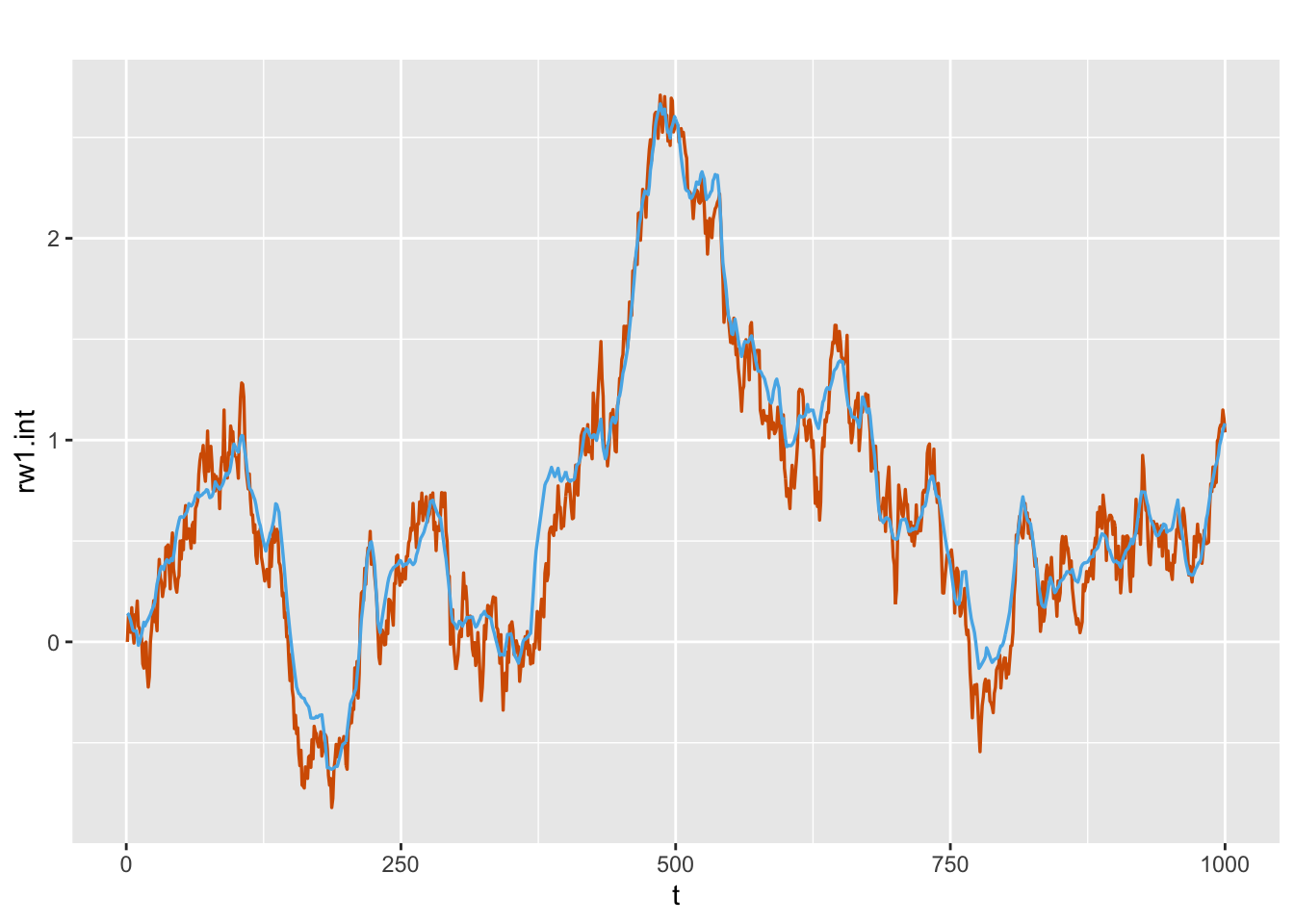
FIGURE 8.5: Actual values (red) and estimated (blue) random walk series for the dynamic intercept \(\beta_{1,t,0}\) from Model D1.
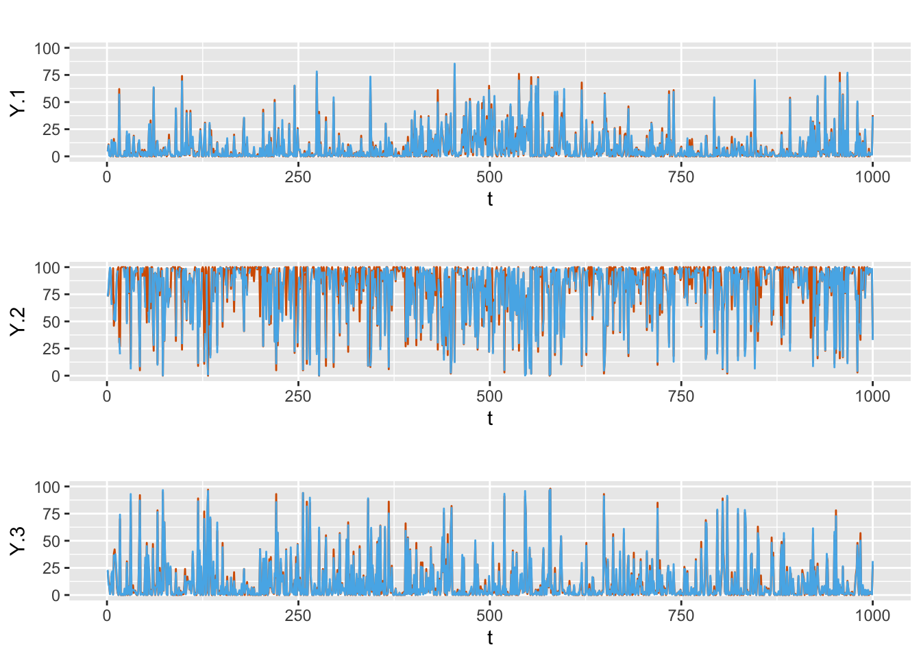
FIGURE 8.6: Actual values (red) and fitted (blue) responses from Model D1.
Alternately, we can include the random intercept only in \(\eta_{2,t}\) (Model D2) or only in \(\eta_{3,t}\) (Model D3) instead of \(\eta_{1,t}\). The in-sample MAEs for these situations are shown in Table 8.1. Detailed code can be seen in the GitHub link for the book.
Model D4: Dynamic coefficient for \(C_{j,t}\)
Consider the model with
\[\begin{align} \eta_{j,t} & = \beta_t C_{j,t} + \delta_j U_{j,t},~j=1,\ldots,3 \tag{8.11} \end{align}\] where the dynamic coefficient \(\beta_t\) evolves as a random walk
\[\begin{align} \beta_{t,0} = \beta_{t-1,0} + w_{t}, \tag{8.12} \end{align}\] with \(w_{t} \sim N(0, \sigma^2_w)\). We use the same true values of \(\delta_j\), \(C_{j,t}\) and \(U_{j,t}\) as before for the simulation. We source the function below for generating the multinomial responses corresponding to the model (8.11) and (8.12).
Multinom.sample.rand <- function(N, rw1.beta) {
  Y <- matrix(NA, ncol = 3, nrow = n)
  eta.1 <- eta.2 <- eta.3 <- rep(NA,n)
  for (t in 1:n) {
    eta.1[t] <- rw1.beta[t] * C.1[t] + deltas[1] * U.1[t]
    eta.2[t] <- rw1.beta[t] * C.2[t] + deltas[2] * U.2[t]
    eta.3[t] <- rw1.beta[t] * C.3[t] + deltas[3] * U.3[t]
    probs <- c(eta.1[t], eta.2[t], eta.3[t])
    probs <- exp(probs) / sum(exp(probs))
    samp <- rmultinom(1, N, prob = probs)
    Y[t,] <- as.vector(samp)
  }
  colnames(Y) <- c("Y.1", "Y.2", "Y.3")
  return(Y)
}
We first generate a random walk series corresponding to rw1.beta. We then compute and plot the response series (plots are not shown here).
rw1.beta <- rep(NA, n)
rw1.beta[1] <- 0
for (t in 2:n) {
  rw1.beta[t] <- rnorm(1, mean = rw1.beta[t - 1], sd = 0.1)
}
N <- 100
Y.rw1 <- Multinom.sample.rand(N, rw1.beta)
df.rw1 <- cbind.data.frame(Y.rw1, C.1, C.2, C.3, U.1, U.2, U.3)
We construct necessary indexes and the data frame as shown below.
Y.new <- c(Y.rw1[,1], Y.rw1[, 2], Y.rw1[, 3])
C.new <- c(df.rw1$C.1, df.rw1$C.2, df.rw1$C.3)
C.1.new <- c(C.1, rep(NA, 2*n))
C.2.new <- c(rep(NA, n), C.2, rep(NA, n))
C.3.new <- c(rep(NA, 2*n), C.3)
C.new <- c(C.1, C.2, C.3)
U.1.new <- c(U.1, rep(NA, 2*n))
U.2.new <- c(rep(NA, n), U.2, rep(NA, n))
U.3.new <- c(rep(NA, 2*n), U.3)
id.rw <- phi.new <- c(rep(1:n, 3))
rw1.idx <- c(1:n, rep(NA, 2*n))
rw2.idx <- c(rep(NA, n), 1:n, rep(NA, n))
rw3.idx <- c(rep(NA, 2*n), 1:n)
re.idx <- rep(1, (3*n))
id.re <- rep(1:n, 3)
inla.dat <- data.frame(Y.new, C.new, C.1.new, C.2.new, C.3.new,
                       U.1.new, U.2.new, U.3.new,
                       phi.new, id.rw, re.idx, id.re,
                       rw1.idx, rw2.idx, rw3.idx)
The formula and inla() call are shown below, followed by a summary of results.
formula.rw1 <- Y.new ~ -1  + U.1.new + U.2.new + U.3.new +
  f(phi.new, model = "iid",
    hyper = list(prec = list(initial = -10, fixed = TRUE))) +
  f(id.rw, C.new, model = "rw1", constr = FALSE) +
  f(
    id.re,
    model = "iid",
    replicate = re.idx,
    hyper = list(theta = list(initial = 20, fixed = T))
  )
model.rw1 <- inla(
  formula.rw1,
  family = "poisson",
  data = inla.dat,
  control.predictor = list(compute = TRUE),
  control.compute = list(dic = TRUE, cpo = TRUE, waic = TRUE)
)
#summary(model.rw1)format.inla.out(model.rw1$summary.fixed[,c(1:5)])
## name mean sd 0.025q 0.5q 0.975q
## 1 U.1.new 1.018 0.046 0.927 1.018 1.109
## 2 U.2.new 3.975 0.039 3.899 3.975 4.051
## 3 U.3.new 2.966 0.033 2.902 2.966 3.030
format.inla.out(model.rw1$summary.hyperpar[,c(1:2)])
## name mean sd
## 1 Precision for id.rw 116.9 10.01The fixed and random coefficients are recovered well by the model fit. We can also plot the simulated and fitted values for the dynamic coefficient \(\beta_t\) as shown in Figure 8.7 below.
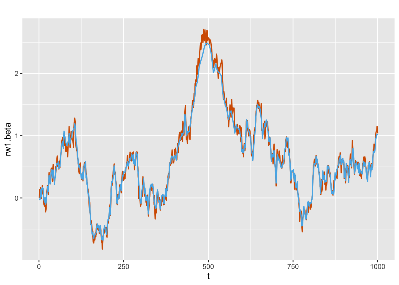
FIGURE 8.7: Actual values (red) and estimated (blue) random walk series for \(\beta_t\) from Model D4.
Plots of the observed and fitted responses are shown in Figure 8.8. In-sample MAEs from all four models, Model D1–D4, are shown in Table 8.1, suggesting that Model D4 performs the best.
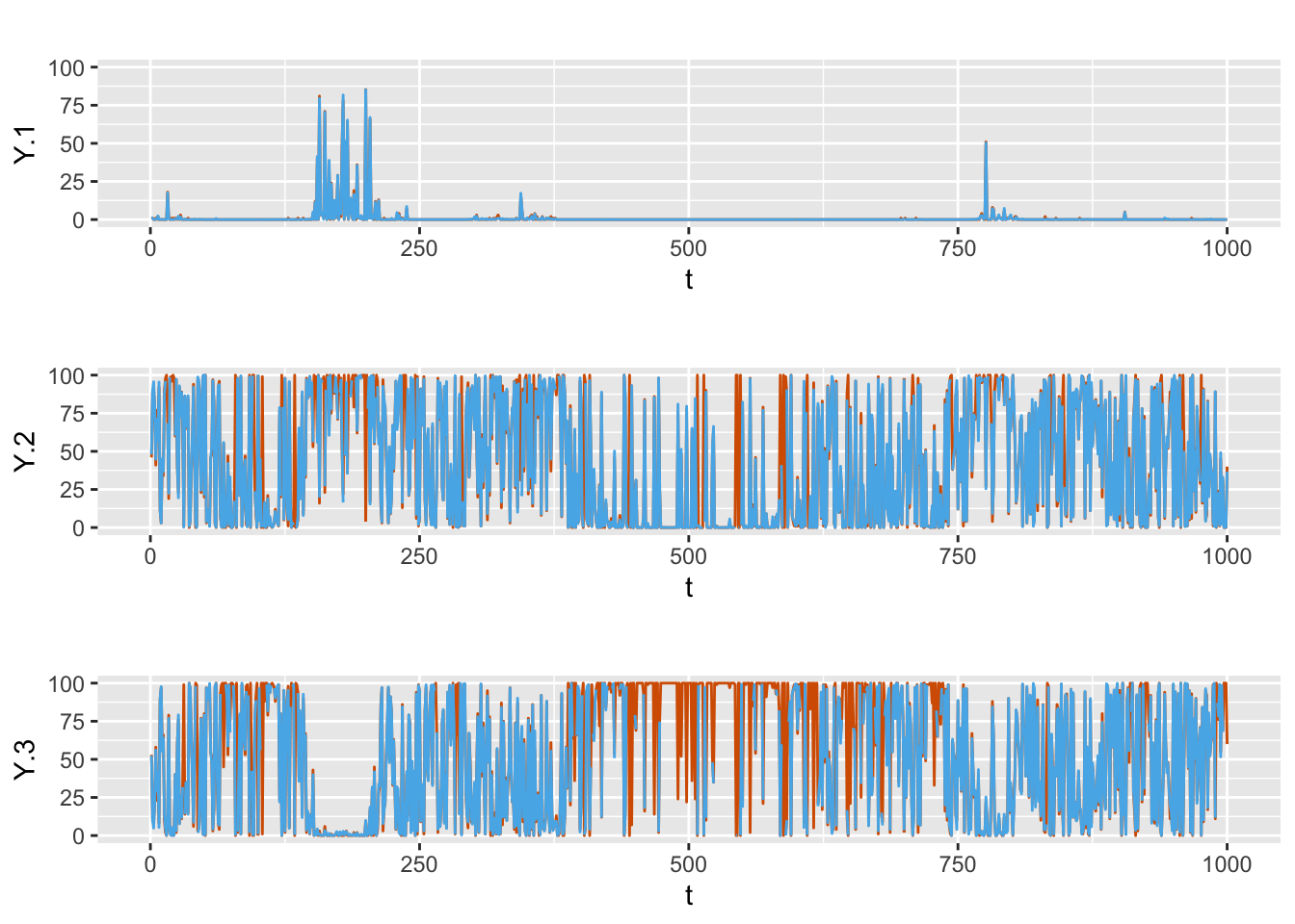
FIGURE 8.8: Actual values (red) and fitted (blue) responses from Model D4.
| Model | MAE(Y.1) | MAE(Y.2) | MAE(Y.3) |
|---|---|---|---|
| D1 | 1.362 | 2.058 | 1.551 |
| D2 | 0.852 | 1.492 | 1.278 |
| D3 | 1.034 | 1.969 | 1.665 |
| D4 | 0.151 | 1.383 | 1.352 |
Chapter 8 – Appendix
Poisson-trick for multinomial models
Given the multinomial likelihood in (8.6), assume that \(Y_{t+}\) is a random variable with Poisson p.m.f. given in (8.7). For \(t=1,\ldots,n\), we can write
\[\begin{align} P(\boldsymbol{y}_t, Y_{t+}=y_{t+}) = P(Y_{t+}=y_{t+}) P(\boldsymbol{y}_t |Y_{t+}=y_{t+}), \tag{8.13} \end{align}\] where the first expression on the right side is given by (8.7) and the second expression, by (8.4). The marginal p.m.f. of \(\boldsymbol{y}_t\) can be obtained by summing the joint p.m.f. in (8.13) over all possible values of \(Y_{t+}\) to yield the Poisson likelihood (which was given in (8.8)):
\[\begin{align*} L_{\mathcal{P}}(\boldsymbol{\phi},\boldsymbol{\beta}; \boldsymbol{Y}^n) \propto \prod_{t=1}^n \prod_{j=1}^J [g_{j,t}(\boldsymbol{\beta}) e^{\phi_t}]^{y_{j,t}} \exp [- g_{j,t}(\boldsymbol{\beta}) e^{\phi_t}]. \end{align*}\]
Let
\[\begin{align} {\widehat{\boldsymbol\phi}} (\boldsymbol{\beta}) = \underset{\boldsymbol \phi}{\text{arg max}}\ L_{\mathcal{P}}(\boldsymbol{\phi},\boldsymbol{\beta}; \boldsymbol{Y}^n) \tag{8.14} \end{align}\] denote the maximum of the profile likelihood function of \(\boldsymbol{\phi}\) given \(\boldsymbol{\beta}\). It can be shown that for \(t=1,\ldots,n\),
\[\begin{align} \widehat{\phi}_t (\boldsymbol{\beta})=\frac{y_{t+}}{G_t(\boldsymbol{\beta})}. \tag{8.15} \end{align}\]
Substituting \(\widehat{\phi}_t (\boldsymbol{\beta})\) from (8.15) into (8.8), we can write (8.8) as a function of only \(\boldsymbol{\beta}\), and show that the resulting expression \(L_{\mathcal{P}}(\boldsymbol{\beta}; \boldsymbol{Y}^n)\) is equivalent to \(L_{\mathcal{M}}(\boldsymbol{\beta}; \boldsymbol{Y}^n)\). It follows that estimation based on \(L_{\mathcal{P}}(\boldsymbol{\phi, \beta}; \boldsymbol{Y}^n)\) and \(L_{\mathcal{M}}(\boldsymbol{\beta}; \boldsymbol{Y}^n)\) will be identical.