Chapter 10 Modeling Stochastic Volatility
10.1 Introduction
An important task in analyzing financial data involves fitting models to study the volatility of asset returns. The class of autoregressive conditionally heteroscedastic (ARCH) models was proposed by Engle (1982), and was extended by Bollerslev (1986) to generalized ARCH (GARCH) models. The simple ARCH(1) model for time series of returns \(r_t\) has the form
\[\begin{align} r_t &= \sigma_t \varepsilon_t, \notag \\ \sigma^2_t &= \alpha_0 + \alpha_1 r^2_{t-1}, \tag{10.1} \end{align}\]
where \(\sigma^2_t\) is the conditional variance of \(r_t\) given the past history \(\{r_{t-1}, r_{t-2},\ldots\}\), \(\alpha_0 >0\), \(0 \le \alpha_1 < 1\), and \(\varepsilon_t\) is an i.i.d. process with mean \(0\) and variance \(1\). The GARCH(1,1) model generalizes the ARCH(1) model and is given by
\[\begin{align} r_t &= \sigma_t \varepsilon_t, \notag \\ \sigma^2_t &= \alpha_0 +\alpha_1 r^2_{t-1} + \beta_1 \sigma^2_{t-1}, \tag{10.2} \end{align}\] where \(\alpha_0 >0\), and \(\alpha_1 + \beta_1 <1\). These models are sometimes called singly stochastic models in the literature because they only have one error \(\varepsilon_t\) in the multiplicative model equation for \(r_t\), but no error in the model for the latent conditional variances \(\sigma^2_t\). The GARCH\((m,r)\) model generalizes these models to include \(m\) ARCH and \(r\) GARCH coefficients. There is an enormous literature on such models, especially in the econometrics domain.
The stochastic volatility (SV) models that were introduced by Taylor (1982) are alternatives to GARCH models and are widely used for modeling volatility in financial time series. SV models introduce an additional error in the (state) model for the latent conditional variance \(\sigma^2_t\), and are referred to in the literature as doubly stochastic models. This chapter describes a state space formulation for SV modeling of a time series.
We source the custom functions.
source("functions_custom.R")This chapter uses the following packages.
library(quantmod)
library(INLA)
library(tidyverse)
library(astsa)
library(gridExtra)
We analyze the following data.
IBM returns from 2018-01-01 to 2020-12-31.
NYSE returns from the
Rpackageastsa.
10.2 Univariate SV models
Jacquier, Polson, and Rossi (1994)
described dynamic Bayesian modeling of an SV model.
We follow the notation in Martino et al. (2011), who described fitting SV models using R-INLA.
The SV model for asset returns \(r_t\) is defined by
\[\begin{align}
r_t &= \exp(h_t/2)\varepsilon_t, \notag \\
h_t -\mu & = \phi(h_{t-1}-\mu) + \sigma_w w_t,
\tag{10.3}
\end{align}\]
where \(h_t\) is the unobserved log volatility, \(\varepsilon_t\) and \(w_t\) are i.i.d. N\((0,1)\) random errors which are independent of each other, \(|\phi| <1\), and \(\mu \in \mathbb{R}\). The model assumes that the latent log volatility \(h_t\) follows a stationary AR(1) process.
Following the discussions in
Martino et al. (2011), we assume a normal prior with mean \(0\) and
a large variance for \(\mu\), an inverse Gamma prior for \(\sigma^2_w\), while
\(\phi\) has the usual logit prior.
The following example illustrates the use of the family="stochvol" option for data simulated from an SV model with \(\varepsilon_t \sim N(0,1)\).
10.2.1 Example: Simulated SV data with standard normal errors
We simulate a time series following (10.3); see inla.doc("stochvol"). Here, \(\varepsilon_t \sim N(0,1)\), as indicated by ret <- exp(h/2) * rnorm(n). The parameter \(\phi = 0.9\) generates a series with high persistence.
set.seed(1234)
n <- 1000
phi <- 0.9
mu <- -2.0
h <- rep(mu, n)
sigma2.w <- 0.25
prec.x <- prec.state.ar1(sigma2.w, phi)
for (i in 2:n) {
  h[i] <- mu + phi * (h[i - 1] - mu) + rnorm(1, 0, sqrt(sigma2.w))
}
ret <- exp(h/2) * rnorm(n)
We use family = "stochvol" to model the SV model. The results are summarized below.
time <- 1:n
data.sim.sv <- cbind.data.frame(ret = ret, time = time)
formula.sim.sv <- ret ~ 0 + f(time, model = "ar1",
                          hyper = list(prec = list(param=c(1,0.0001)),
                                    mean = list(fixed = FALSE)))
model.sim.g <-
  inla(formula.sim.sv, family = "stochvol", data = data.sim.sv,
         control.compute = list(
    dic = TRUE,
    waic = TRUE,
    cpo = TRUE,
    config = TRUE),
  )
#summary(model.sim.g)
format.inla.out(model.sim.g$summary.hyperpar[c(1,2)])
##   name               mean   sd
## 1 Precision for time  0.949 0.151
## 2 Rho for time        0.888 0.026
## 3 Mean for time      -2.133 0.139
Note that the mean \(\mu\) of the log volatility \(h_t\) in the latent AR(1) state equation (10.3) is recovered from the estimate of “Mean for time” in the output, with posterior mean
\(- 2.133\)
and posterior standard deviation 0.139.
If there are exogenous predictors, we can replace model = "ar1" by model = "ar1c".
10.2.2 Example: Simulated SV data with Student-\(t_{\nu}\) errors
The model generating mechanism is the same as in the previous example, except for assuming that
\(\varepsilon_t \sim t_\nu\), i.e., a Student-\(t\) distribution with \(\nu\) degrees of freedom (d.f.), \(\nu\) being treated as an unknown parameter. The \(t\)-distribution allows for heavier tails than the normal and is widely used in modeling financial data (Tsay 2005). The use of stochvol_t enables us to adequately recover the true values.
The dof-prior has a tabulated density and is the PC prior for the degrees of freedom parameter in the Student-t distribution (see Section 3.9.2). The parameters of this prior are \((u, \alpha)\) with the interpretation that \(P(\nu < u) = \alpha\). The code for data generation is the same as the code for the Gaussian case, except for replacing
ret <- exp(h/2) * rnorm(n)by
ret <- exp(h / 2) *rt(n, df=5)The code for the formula and model fit are also similar to the Gaussian case, except for replacing
family = "stochvol" by family = "stochvol_t" in the inla() call.
format.inla.out(model.sim.t$summary.hyperpar[c(1,2,4)])
##   name                                      mean   sd    0.5q
## 1 degrees of freedom for stochvol student-t 12.477 8.800  9.841
## 2 Precision for time                         0.837 0.161  0.826
## 3 Rho for time                               0.875 0.037  0.881
## 4 Mean for time                             -1.796 0.162 -1.792
10.2.3 Example: IBM stock returns
We download daily prices \(P_t\) for IBM using the R package
quantmod, and compute the returns as
\(r_t = \nabla \log P_t = (1-B)\log P_t\), where \(B\) is the backshift operator.
The IBM price data from 2018-01-01 to 2020-12-31 is shown in
Figure 10.1, together with the returns (we dropped the first NA).
library(gridExtra)
getSymbols(
  "IBM",
  from = '2018-01-01',
  to = "2020-12-31",
  warnings = FALSE,
  auto.assign = TRUE
)
## [1] "IBM"
ret <- ts(diff(log(IBM$IBM.Adjusted)))[-1]
adj.plot <-
  tsline(
    as.numeric(IBM$IBM.Adjusted),
    xlab = "t",
    ylab = "Adjusted price",
    line.color = "black",
    line.size = 0.6
  )
ret.plot <- tsline(
  ret,
  xlab = "t",
  ylab = "Returns",
  line.color = "red",
  line.size = 0.6
)
grid.arrange(adj.plot, ret.plot, nrow = 1)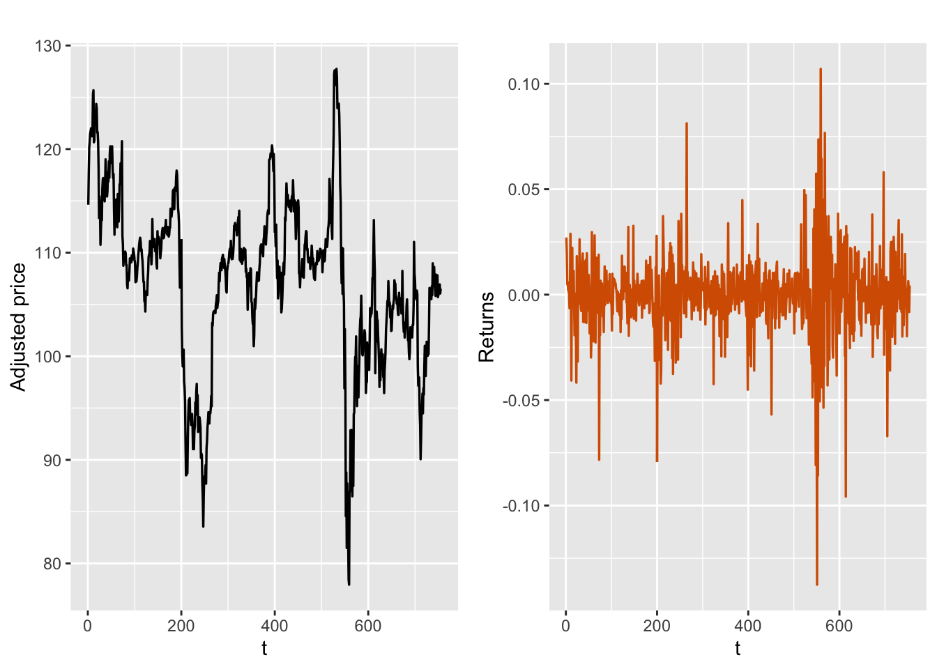
FIGURE 10.1: Adjusted prices (left) and log returns (right) for IBM.
We fit the univariate SV model discussed in (10.3) to the time series of length \(n=754\) of daily returns for IBM, assuming three different possible distributions for \(\varepsilon_t\). The option family = "stochvol" fits an SV model (10.3) with i.i.d. N(0,1) errors \(\varepsilon_t\).
set.seed(1234)
id.1 <- 1:length(ret)
data.ret <- cbind.data.frame(ret, id.1)
formula.ret <- ret ~ 0 + f(id.1,model="ar1",
                       hyper = list(prec = list(param=c(1,0.0001)),
                                    mean = list(fixed = FALSE)))
model.g <- inla(
  formula.ret,
  family = "stochvol",
  data = data.ret,
  control.compute = list(
    dic = TRUE,
    waic = TRUE,
    cpo = TRUE,
    config = TRUE
  ),
  control.predictor = list(compute = TRUE, link = 1)
)
#summary(model.g)
format.inla.out(model.g$summary.hyperpar[c(1,2,4)])
##   name               mean   sd    0.5q
## 1 Precision for id.1  0.038 0.020  0.035
## 2 Rho for id.1        0.998 0.001  0.998
## 3 Mean for id.1      -0.439 0.675 -0.464
The estimated posterior mean of \(\phi\) is 0.998, which indicates very high persistence. Note that summary.fitted.values gives the fitted values of \(\sigma^2_t\).
We can obtain fitted values of \(\exp(h_t)\)
using summary.linear.predictor.
We overlay a plot of the squared returns \(r_t^2\) and the posterior mean of \(\exp(h_t)\); see the top panel of Figure 10.2.
fit.model.g <- exp(model.g$summary.linear.predictor$mean) If we suspect that the assumption of standard normal errors \(\varepsilon_t\) may not be suitable, we can also fit a model with i.i.d. Student-\(t\) errors by
replacing family = "stochvol" in the model.g call above by
family = "stochvol_t" in model.t. The results are shown below.
#summary(model.t)
format.inla.out(model.t$summary.hyperpar[c(1,2)])
##   name                                      mean   sd
## 1 degrees of freedom for stochvol student-t  5.842 1.225
## 2 Precision for id.1                         0.055 0.034
## 3 Rho for id.1                               0.999 0.001
## 4 Mean for id.1                             -0.541 0.878
fit.model.t <-
exp(model.t$summary.linear.predictor$mean) The high value of the estimated \(\phi\) indicates a high degree of persistence. The estimated d.f. for the \(t\)-distribution is about \(6\). Again, the fitted means of \(\exp(h_t)\) are obtained as shown earlier for model.g. A plot of these values and \(r_t^2\) is shown in the lower plot in Figure 10.2.
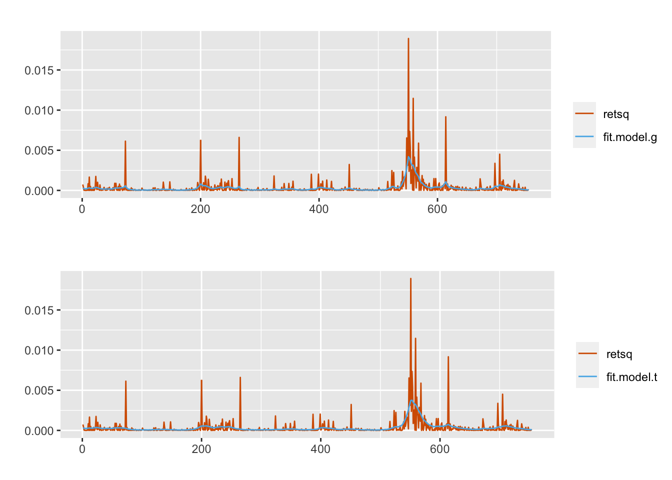
FIGURE 10.2: Comparing observed squared returns (red) and fitted squared volatilities (blue) from the two models for the IBM data.
We note that due to Monte Carlo sampling which INLA uses internally, there are likely to be small differences in the results when running family = stochvol_t on different computers. But overall, the results should be more or less the same (in terms of reproducibility). Martino et al. (2011) also describe how to use family = "stochvol_nig" for SV modeling where \(\varepsilon_t\) follows a normal inverse Gaussian distribution. See Barndorff-Nielsen (1997) and Andersson (2001) who described the NIG distribution as a variance-mean mixture of a normal distribution with the inverse Gaussian distribution as the mixing distribution. We refer the reader to Martino et al. (2011) for more details.
Table 10.1 shows the DIC, WAIC, and the marginal likelihoods for the two models. They are very close, with the values for model.t being slightly better.
| Model | DIC | WAIC | Marginal Likelihood |
|---|---|---|---|
| model.g | \(-4262.231\) | \(-4238.848\) | \(2070.688\) |
| model.t | \(-4260.187\) | \(-4259.245\) | \(2084.247\) |
10.2.4 Example: NYSE returns
To illustrate the approach on a longer time series, we run these codes on the nyse data of length \(n=2000\) from the R package astsa. We are able to closely recover estimates of \(\sigma_w\) and \(\phi\) from family = "stochvol_t", which were similar to the results in Shumway and Stoffer (2017); however, unlike their setup, we do not include an \(\alpha\) in the observation level equation, but only include a state level mean \(\mu\).
id.1 <- 1:length(nyse)
data.nyse <- cbind.data.frame(nyse, id.1)
formula.nyse <- nyse ~ 0 + f(id.1,model="ar1",
                       hyper = list(prec = list(param=c(1,0.001)),
                                    mean = list(fixed = FALSE)))
model.nyse <- inla(
  formula.nyse,
  family = "stochvol_t",
  data = data.nyse,
  control.compute = list(
    dic = TRUE,
    waic = TRUE,
    cpo = TRUE,
    config = TRUE
  ),
  control.predictor = list(compute = TRUE, link = 1)
)
#summary(model.nyse)
format.inla.out(model.nyse$summary.hyperpar[,c(1:2)])
##   name                                      mean   sd
## 1 degrees of freedom for stochvol student-t  5.144 0.664
## 2 Precision for id.1                         2.269 0.984
## 3 Rho for id.1                               0.994 0.005
## 4 Mean for id.1                             -9.048 0.335