Chapter 5 Time Series Regression Models
5.1 Introduction
This chapter discusses time series regression models. The response is a univariate time series that we wish to model and forecast. We discuss two types of predictors: (a) predictors that we construct as functions of time and include in a structural decomposition model, and (b) exogenous time series that are observed on the same time frame and may be associated with the response time series at contemporaneous or lagged times. We also show how we can build a latent AR(1) model with fixed, exogenous predictors.
As in previous chapters, the custom functions must be sourced.
source("functions_custom.R")The list of packages used in this chapter are shown below.
library(INLA)
library(astsa)
library(lubridate)
library(tidyverse)
library(gridExtra)
We show analyses for the following data.
Monthly average cost of nightly hotel stay
Hourly traffic volumes
5.2 Structural models
This section casts the well known structural decomposition of a univariate time series as a dynamic linear model (DLM) and shows how to fit and forecast the time series using R-INLA. An observed time series may exhibit features such as trend and seasonality, in addition to stochastic dependence. To build a structural time series model (also called a classical decomposition model in the literature), we decompose a time series \(y_t\) as the sum of different components:
\[\begin{align} y_{t} &= \mbox{Level + Trend + Seasonal Component + Random Component},~ i.e., \notag \\ y_{t} &= \alpha + m_{t} + S_{t} + v_{t}, \tag{5.1} \end{align}\] where \(\alpha\) is a level coefficient, \(m_{t}\) denotes a latent trend component, \(S_{t}\) denotes a latent seasonal component, and \(v_{t}\) denotes a random error component. The seasonal period is an integer such as \(s= 4, 7\), or \(12\), corresponding to time series that exhibits a quarterly, daily, or monthly effect. The structural decomposition models have wide application in business, economics, etc.; see Harvey and Koopman (2014).
5.2.1 Example: Monthly average cost of nightly hotel stay
The data consists of the monthly average cost of a night’s accommodation at a hotel, motel or guesthouse in Victoria, Melbourne, from January 1980 to June 1995. In Figure 5.1, we show plots of the time series (cost), as well as the natural logarithm of the series (lcost). The plot of the nonstationary time series lcost stabilizes the variance in cost, and exhibits an increasing trend.
hotels <- read.csv("NightlyHotel.csv")
str(hotels)
## 'data.frame':    186 obs. of  3 variables:
##  $ Yr_mth: chr  "1980-01" "1980-02" "1980-03" "1980-04" ...
##  $ Cost  : num  27.7 28.7 28.6 28.3 28.6 ...
##  $ CPI   : num  45.2 45.2 45.2 46.6 46.6 46.6 47.5 47.5 47.5 48.5 ...
cost <- ts(hotels[, 2])
lcost <- log(cost)
c1 <-
  tsline(
    as.numeric(cost),
    xlab = "Month",
    ylab = "cost",
    line.size = 0.6,
    line.color = "black"
  )
lc1 <-
  tsline(
    as.numeric(lcost),
    xlab = "Month",
    ylab = "log cost",
    line.size = 0.6,
    line.color = "red"
  )
grid.arrange(c1, lc1, nrow = 1)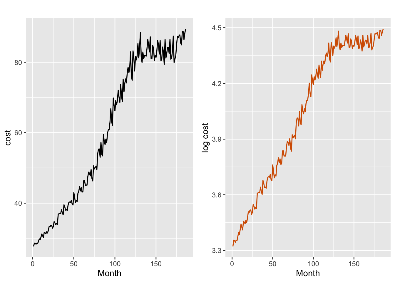
FIGURE 5.1: Average monthly cost (left plot) and log cost (right plot).
We fit a DLM to the nonstationary series lcost to handle the time-varying trend with additive seasonality (with \(s = 12\)), deferring a discussion of conditional heteroscedasticity until Chapter 10.
Keeping in mind that R-INLA has no predict function, we must append the training data with NA’s to represent the hold-out times. We hold out six months of data for predictive cross validation.
Each of the vectors trend and y.append has length \(n=186\), with \(n_t=180\) and \(n_h=6\) denoting the training and hold-out samples respectively. We bind these columns to create a data frame.
n <- length(lcost)
n.hold <- 6
n.train <- n - n.hold
test.lcost <- tail(lcost, n.hold)
train.lcost <- lcost[1:n.train]
y <- train.lcost
y.append <- c(y, rep(NA, n.hold))
n.seas <- 12
trend <- 1:length(y.append)
lcost.dat <- cbind.data.frame(y = y.append,
                              trend = trend,
                              seasonal = trend)
We model the latent trend \(m_t\) by a random walk
\[\begin{align} m_{t} = m_{t-1} + w_{t,1}, \tag{5.2} \end{align}\] where \(w_{t,1}\) is a Gaussian state error process. The seasonal variation in lcost with periodicity \(s=12\) can be modeled by assuming that \(\sum_{j=0}^{s-1} S_{t-j}\) are independent Gaussian random variables, i.e.,
\[\begin{align}
S_t = -\sum_{j=1}^{11}S_{t-j} + w_{t,2}. \tag{5.3}
\end{align}\]
For details, see inla.doc("seasonal"). Equations (5.2) and (5.3) are the state equations in the DLM for lcost, while the observation equation is
given by (5.1). When we fitted a model with level \(\alpha\), we saw that this coefficient was not significant. We therefore show the code and results for a model without level \(\alpha\).
formula.lcost.rw1 <- y.append ~ -1 +
  f(trend, model = "rw1", constr = FALSE) +
  f(seasonal, model = "seasonal",
    season.length = n.seas)
model.lcost.rw1 <- inla(
  formula.lcost.rw1,
  family = "gaussian",
  data = lcost.dat,
  control.predictor = list(compute = TRUE),
  control.compute = list(
    dic = TRUE,
    waic = TRUE,
    cpo = TRUE,
    config = TRUE
  )
)
summary(model.lcost.rw1)
##
## Call:
##    c("inla(formula = formula.lcost.rw1, family = \"gaussian\",
##    data = lcost.dat, ", " control.compute = list(dic = TRUE, waic
##    = TRUE, cpo = TRUE, ", " config = TRUE), control.predictor =
##    list(compute = TRUE))" )
## Time used:
##     Pre = 4.57, Running = 0.315, Post = 0.249, Total = 5.13
## Random effects:
##   Name     Model
##     trend RW1 model
##    seasonal Seasonal model
##
## Model hyperparameters:
##                                             mean       sd 0.025quant
## Precision for the Gaussian observations 38811.25 21587.79   12937.41
## Precision for trend                      3937.54   636.43    2821.77
## Precision for seasonal                  55786.67 18354.44   28280.75
##                                         0.5quant 0.975quant     mode
## Precision for the Gaussian observations 33678.14   94599.50 25854.69
## Precision for trend                      3891.96    5320.38  3806.62
## Precision for seasonal                  52980.47   99654.59 47811.14
##
## Expected number of effective parameters(stdev): 157.84(9.71)
## Number of equivalent replicates : 1.14
##
## Deviance Information Criterion (DIC) ...............: -1202.97
## Deviance Information Criterion (DIC, saturated) ....: 334.93
## Effective number of parameters .....................: 156.14
##
## Watanabe-Akaike information criterion (WAIC) ...: -1227.92
## Effective number of parameters .................: 98.53
##
## Marginal log-Likelihood:  387.22
## CPO and PIT are computed
##
## Posterior marginals for the linear predictor and
##  the fitted values are computed
To see all the items in the list summary(model.lcost.rw1), we can use
names(summary(model.lcost.rw1))
##  [1] "call"             "cpu.used"         "hyperpar"
##  [4] "random.names"     "random.model"     "neffp"
##  [7] "dic"              "waic"             "mlik"
## [10] "cpo"              "linear.predictor" "family"
The condensed output for the random effects is shown below.
format.inla.out(model.lcost.rw1$summary.hyperpar[,c(1:2)])## name mean sd
## 1 Precision for Gaussian obs 38811 21587.8
## 2 Precision for trend 3938 636.4
## 3 Precision for seasonal 55787 18354.4Plots of the posterior means of \(m_t\) and \(S_t\) along with the sample spectrum, ACF, and PACF of \(S_t\) in Figure 5.2 show evidence of periodic behavior with \(s=12\).
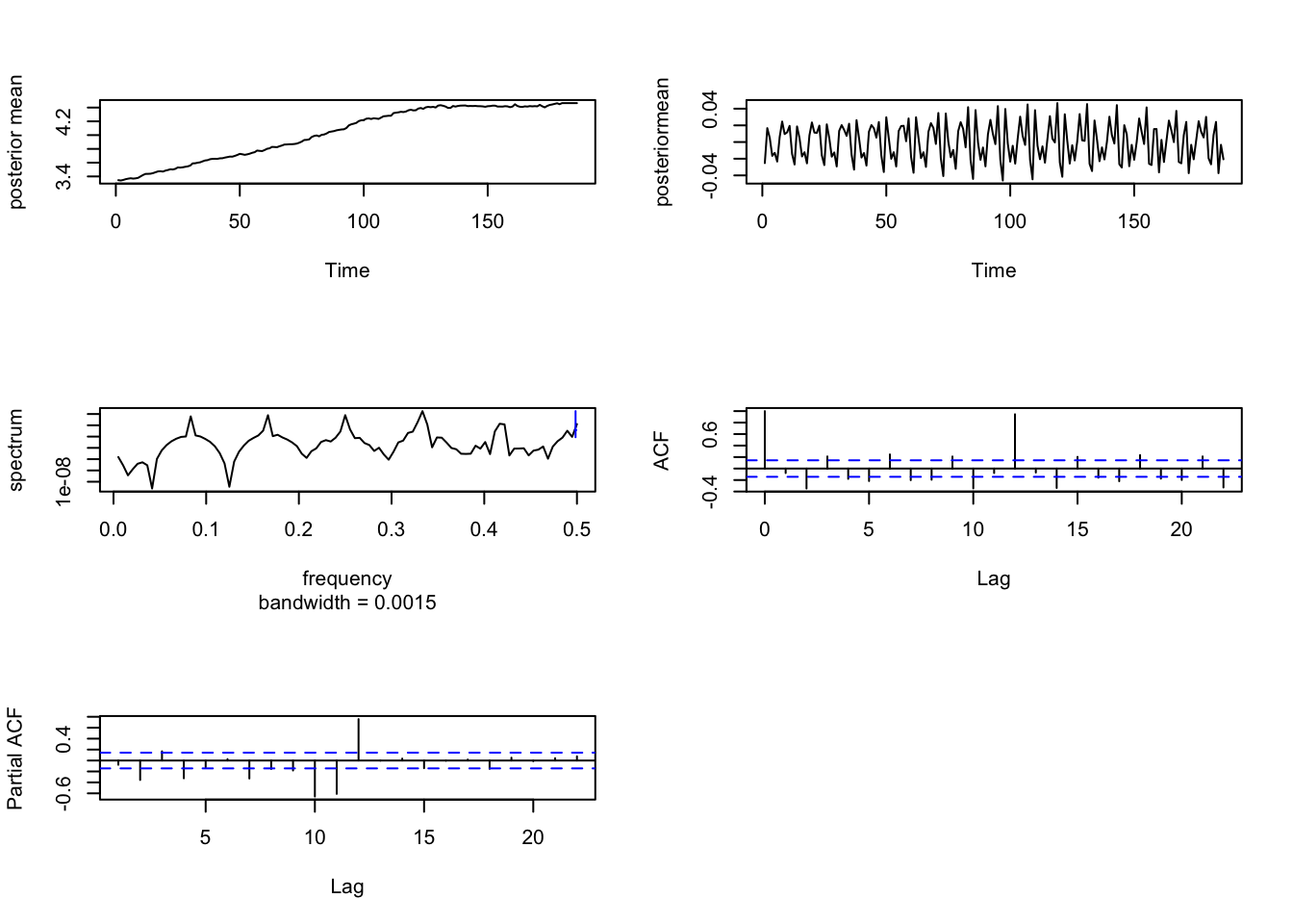
FIGURE 5.2: The top plot (left panel) shows the posterior means of \(m_t\), while the top plot (right panel) is the posterior mean of \(S_t\). The plot in the middle (left panel) is the spectrum of the posterior means of \(S_t\), the plot in the middle (right panel) is the ACF of the posterior means of \(S_t\), and the plot in the bottom (left panel) is the PACF of \(S_t\).
The marginal likelihood, DIC, and WAIC are shown below:
summary(model.lcost.rw1)$mlik
##                                        [,1]
## log marginal-likelihood (integration) 387.3
## log marginal-likelihood (Gaussian)    387.2
summary(model.lcost.rw1)$dic$dic
## [1] -1203
summary(model.lcost.rw1)$waic$waic
## [1] -1228
We can obtain forecasts for future state variables, \(m_{n_t+\ell}\) and \(S_{n_t+\ell}\), for \(\ell=1,\ldots, n_h\).
format.inla.out(tail(model.lcost.rw1$summary.random$trend, n.hold)[,c(2:6)])
##   name mean  sd    0.025q 0.5q  0.975q
## 1 181  4.465 0.019 4.428  4.465 4.502
## 2 182  4.465 0.025 4.416  4.465 4.513
## 3 183  4.465 0.029 4.407  4.465 4.523
## 4 184  4.465 0.034 4.399  4.465 4.531
## 5 185  4.465 0.037 4.392  4.465 4.538
## 6 186  4.465 0.041 4.385  4.465 4.545
format.inla.out(tail(model.lcost.rw1$summary.random$seasonal,
                     n.hold)[,c(2:5)])
##   name mean   sd   0.025q 0.5q
## 1 181  -0.027 0.01 -0.046 -0.027
## 2 182   0.008 0.01 -0.012  0.008
## 3 183   0.024 0.01  0.004  0.024
## 4 184  -0.037 0.01 -0.057 -0.037
## 5 185  -0.003 0.01 -0.023 -0.003
## 6 186  -0.021 0.01 -0.040 -0.021
Forecasts of \(y_{n_t+\ell}\) for \(\ell=1,\ldots,n_h\) can also be obtained.
format.inla.out(tail(model.lcost.rw1$summary.fitted.values,n.hold)[,c(1:5)])
##   name         mean  sd    0.025q 0.5q  0.975q
## 1 fit.Pred.181 4.438 0.022 4.395  4.438 4.482
## 2 fit.Pred.182 4.473 0.027 4.420  4.473 4.526
## 3 fit.Pred.183 4.489 0.031 4.427  4.489 4.551
## 4 fit.Pred.184 4.427 0.035 4.358  4.427 4.497
## 5 fit.Pred.185 4.461 0.039 4.385  4.461 4.538
## 6 fit.Pred.186 4.444 0.042 4.362  4.444 4.527
The MAPE and MAE values corresponding to these forecasts are 0.441 and 0.02 respectively. The fitted lcost time series shown in the left panel of Figure 5.3 indicates a very close fit with the observed series. Both series show a leveling off pattern. The plot also shows the observations and forecasts for the \(n_h = 6\) values of the hold-out sample of lcost. There is some disparity since the observed lcost appears to be increasing in the test portion, while the forecast values continue the leveling off pattern. The right panel shows the corresponding plots for the cost series.
fit.lcost.rw1 <- model.lcost.rw1$summary.fitted.values$mean
plot.data.rw1 <-
  as_tibble(cbind.data.frame(
    time = trend,
    lcost = lcost,
    lcost.fit = fit.lcost.rw1
  ))
p.lcost <- multiline.plot(
  plot.data.rw1,
  xlab = "Month",
  ylab = "",
  line.type = "solid",
  line.size = 0.6,
  line.color = c("red", "blue")
) +
  geom_vline(xintercept = n.train, size = 0.2)
# cost
fit.cost <- exp(fit.lcost.rw1)
plot.data <-
  as_tibble(cbind.data.frame(
    time = trend,
    cost = cost,
    cost.fit = fit.cost
  ))
p.cost <- multiline.plot(
  plot.data,
  xlab = "Month",
  ylab = "",
  line.type = "solid",
  line.size = 0.6,
  line.color = c("red", "blue")
) +
  geom_vline(xintercept = n.train, size = 0.2)
grid.arrange(p.lcost, p.cost, layout_matrix = cbind(1,2))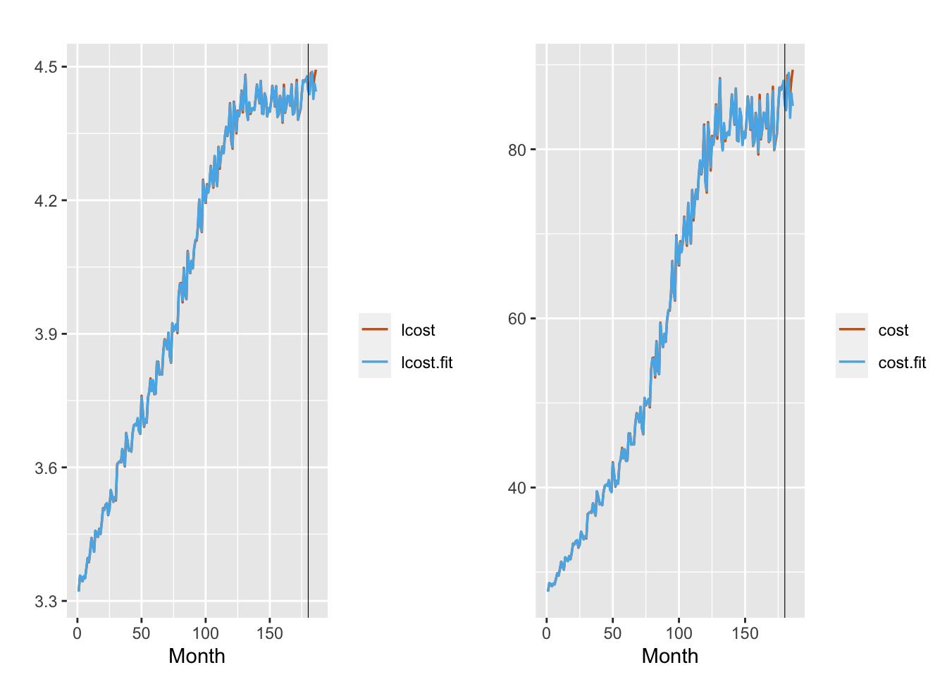
FIGURE 5.3: Observed (red) versus fitted (blue) lcost (left panel) and cost (right panel) from Model 1. The black vertical line divides the data into training and test portions in each plot.
5.3 Models with exogenous predictors
In many situations, we wish to model a time series \(y_t\) as a function of exogenous predictors in addition to functions of time to reflect trend or seasonality. The observation equation of the DLM has \(k\) exogenous variables \(Z_1,\ldots,Z_k\) observed over time in addition to a latent state variable \(x_t\) and additive noise \(v_t\). We treat the regression coefficients \(\beta_1,\ldots,\beta_k\) corresponding to the exogenous variables to be fixed unknown constants. We can assume that the state equation has an AR\((p)\) or random walk structure; here, we show an AR(1) state equation.
\[\begin{align} y_t &= x_t + \sum_{j=1}^k \beta_j Z_{t,j} + v_t;~~ v_t \sim N(0, \sigma^2_v), \tag{5.4}\\ x_t &= \phi x_{t-1} + w_t; ~~ w_t \sim N(0, \sigma^2_w), t=2,\ldots,n; \tag{5.5} \end{align}\] \(x_1\) follows the normal distribution in (3.3), \(\vert \phi \vert <1\), \(Z_{t,j},~j=1,\ldots,k\) are exogenous time series, and \(\beta_j,~j=1,\ldots,k\) are the corresponding regression coefficients.
5.3.1 Example: Hourly traffic volumes
We model hourly traffic volumes data by combining the framework in (5.1) with the equations (5.4)-(5.5). The data is available from the Center for Machine Learning and Intelligent Systems at the University of California website.5 The hourly Interstate 94 Westbound traffic volume was recorded at the Automated Traffic Recording station 301 of Minnesota’s Department of Transportation(DoT) located roughly midway between Minneapolis and St. Paul.
traffic <-
  read.csv(file = "Metro_Interstate_94 Traffic_Volume_Hourly.csv",
           header = TRUE,
           stringsAsFactors = FALSE)
traffic <- as_tibble(traffic)
traffic <- traffic %>%
  mutate(date_time = as.POSIXct(
    as.character(date_time),
    origin = "1899-12-30",
    format = "%m/%d/%Y %H",
    tz = "UTC"
  ))
traffic <- traffic %>%
  mutate(
    month = month(date_time, label = TRUE),
    day = day(date_time),
    year = year(date_time),
    dayofweeek = weekdays(date_time),
    hourofday = hour(date_time),
    weeknum = week(date_time)
  )
We fit models to three months of hourly data (in 1000’s), consisting of \(n=2160\) observations. In Figure 5.4, we show plots of the time series (after normalizing the values by dividing them by 1000), the sample ACF and sample spectrum plotted versus frequency, as well as the amplitudes of the spectrum plotted versus period.
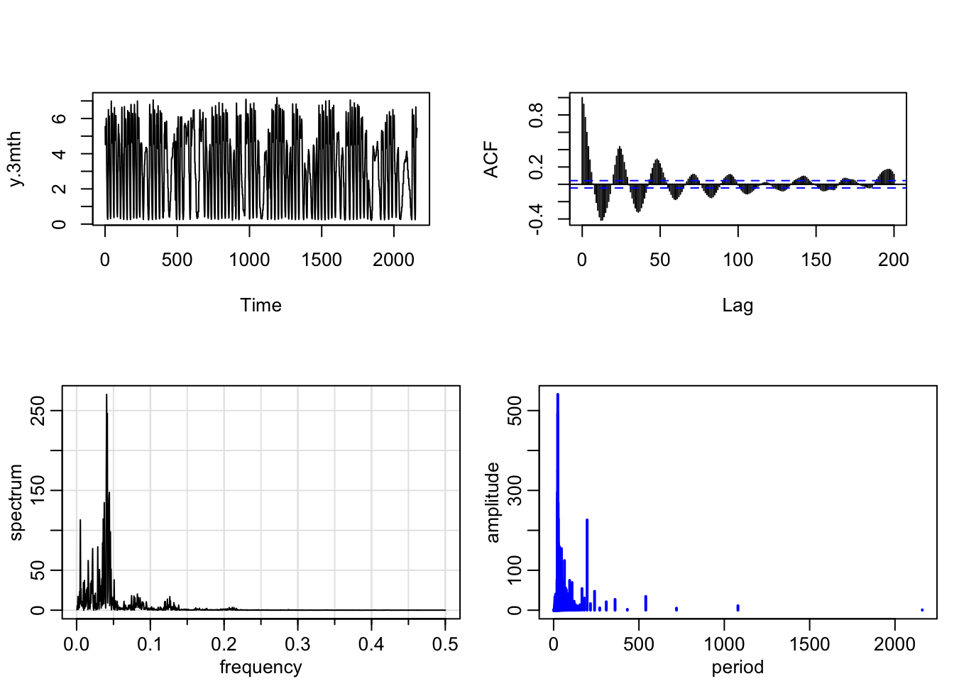
FIGURE 5.4: Time series plot (left) and ACF (right) of hourly traffic volume in the top panel and sample spectrum (left) and amplitude versus period (right) in the bottom panel.
We can identify the periods (or harmonics) associated with the highest periodogram amplitudes. Since this is hourly data, we will expect to see a period of \(24\). From the periodogram, we can see that the highest amplitude is indeed associated with period \(24\) (corresponding to harmonic 90) and values near \(24\). Periods in the vicinity of \(7 \times 24=168\) point to daily periodicity. The sample periodogram points to harmonics in the vicinity of the periods \(168\) and \(196\) as having higher amplitudes. In addition, we can include harmonics with high amplitudes associated with other periods, and create sine and cosine terms associated with these periods that serve as predictors in the DLM.
id <- 1:n
k <- c(90, 11, 20, 47, 62, 23, 9, 34, 29, 13)
sin.mat <- cos.mat <- matrix(0, nrow = n, ncol = length(k))
for (i in 1:length(k)) {
  sin.mat[, i] <- sin(2 * pi * id * k[i] / n)
  colnames(sin.mat) <- paste("S", c(1:(length(k))), sep = "")
  cos.mat[, i] <- cos(2 * pi * id * k[i] / n)
  colnames(cos.mat) <- paste("C", c(1:(length(k))), sep = "")
}
It is also useful to see whether exogenous predictors relating to holiday and weather effects affect the traffic volume.
holiday <- traffic$holiday[1:n]
temp <- traffic$temp[1:n]
rain <- traffic$rain_1h[1:n]
snow <- traffic$snow_1h[1:n]
clouds <- traffic$clouds_all[1:n]
weather <- traffic$weather_main[1:n]
dayofweek <- traffic$dayofweeek[1:n]
hourofday <- traffic$hourofday[1:n]
We set up a data frame with all the variables.
trend <- 1:n
y.traffic <-
  cbind.data.frame(
    y.3mth, id, trend = trend, sin.mat, cos.mat,
    holiday, temp, rain, snow, clouds, weather,
    dayofweek, hourofday
  )
Model E1
We set up and fit a DLM with the leading harmonics as exogenous fixed predictors, and an AR(1) trend. Since we anticipate that the leading harmonics that we obtained empirically will capture significant hourofday and dayofweek effects, we exclude these two variables from the model.
formula.3mth.1 <-
  y.3mth ~ 1 + sin.mat +cos.mat +
f(trend, model = "ar1", constr = FALSE)model.3mth.1 <- inla(
formula.3mth.1,
family = "gaussian",
data = y.traffic,
control.predictor = list(compute = TRUE),
control.compute = list(dic = TRUE, cpo = TRUE, waic = TRUE)
)
#summary(model.3mth.1)The condensed summaries on estimated effects are shown below. If the interval (0.025q, 0.975q) does not include 0, we say that the effect is significant in the Bayesian sense (D. A. Berry 1996).
format.inla.out(model.3mth.1$summary.fixed[,c(1:5)])
##    name      mean   sd    0.025q 0.5q   0.975q
## 1  Intercept  3.274 0.210  2.861  3.273 3.687
## 2  S1         0.447 0.088  0.274  0.447 0.620
## 3  S2        -0.132 0.276 -0.676 -0.132 0.412
## 4  S3         0.138 0.241 -0.336  0.138 0.610
## 5  S4         0.364 0.151  0.067  0.364 0.661
## 6  S5         0.304 0.122  0.065  0.304 0.543
## 7  S6         0.122 0.228 -0.327  0.122 0.570
## 8  S7         0.232 0.283 -0.326  0.232 0.788
## 9  S8        -0.104 0.188 -0.472 -0.104 0.265
## 10 S9         0.096 0.205 -0.307  0.096 0.499
## 11 S10        0.163 0.269 -0.367  0.163 0.692
## 12 C1         0.510 0.088  0.337  0.510 0.683
## 13 C2         0.448 0.274 -0.091  0.448 0.987
## 14 C3        -0.207 0.239 -0.677 -0.207 0.263
## 15 C4        -0.114 0.151 -0.410 -0.114 0.182
## 16 C5         0.241 0.122  0.002  0.241 0.479
## 17 C6         0.249 0.227 -0.198  0.249 0.695
## 18 C7         0.031 0.280 -0.521  0.031 0.583
## 19 C8        -0.314 0.187 -0.681 -0.314 0.053
## 20 C9         0.207 0.204 -0.194  0.207 0.608
## 21 C10        0.184 0.267 -0.341  0.184 0.709
format.inla.out(model.3mth.1$summary.hyperpar[,c(1:2)])
##   name                       mean      sd
## 1 Precision for Gaussian obs 16167.684 1.05e+04
## 2 Precision for trend            0.259 3.00e-02
## 3 Rho for trend                  0.922 9.00e-03
model.3mth.1$mlik
##                                        [,1]
## log marginal-likelihood (integration) -2585
## log marginal-likelihood (Gaussian)    -2587
We note that the cosine/sine pair (C1, S1) corresponding to the period \(24\) definitely contribute to the model. Also significant are S4 and S5 which are associated with (approximately) periods of 46 and 35, which in turn may be related to 2 day and 1.5 day cycles, respectively. The posterior mean of \(\phi_1\) is 0.98. We can also refit the model including the weather related variables; we do not show details here.
Model E2
In Model E2, we include hourofday and dayofweek effects, as well as weather/holiday variables as fixed exogenous predictors, together with an AR(1) trend, but exclude the empirically determined leading harmonics.
formula.3mth.2 <- y.3mth ~ 1 + hourofday + dayofweek +
  holiday + temp + rain + snow + clouds + weather +
  f(trend, model = "ar1", constr = FALSE)
model.3mth.2 <- inla(
  formula.3mth.2,
  family = "gaussian",
  data = y.traffic,
  control.predictor = list(compute = TRUE),
  control.compute = list(
    dic = TRUE,
    cpo = TRUE,
    waic = TRUE,
    config = TRUE
  )
)
format.inla.out(model.3mth.2$summary.hyperpar[,c(1:2)])
##   name                       mean      sd
## 1 Precision for Gaussian obs 21952.358 19432.950
## 2 Precision for trend            0.268     0.028
## 3 Rho for trend                  0.919     0.009
model.3mth.2$mlik  # marginal likelihood
##                                        [,1]
## log marginal-likelihood (integration) -2606
## log marginal-likelihood (Gaussian)    -2606
The DIC, WAIC, and PsBF values from the two models are displayed in Table 5.1. All these criteria prefer Model E2. The setup shown above can be used to investigate other models for the hourly traffic in order to identify the smallest significant model, but the details are not shown here.
| Model | DIC | WAIC | PsBF |
|---|---|---|---|
| Model E1 | \(-12989.964\) | \(-13432.837\) | \(4776.67\) |
| Model E2 | \(-12868.756\) | \(-13308.067\) | \(4719.287\) |
Remark. Frequently, we must model time series exhibiting multiple seasonal periods. For example, the soi data in the R package astsa
exhibits an annual cycle (\(s_1 =12\)) and a four-year cycle (\(s_2 = 48\)).
Call center volume data often exhibit an hour of day effect as well as a weekly, or monthly cycle. In a non-dynamic setting, we can use the msts() function in the R package forecast (R. Hyndman et al. (2021) and R. J. Hyndman and Khandakar (2008)).
Suppose \(s_1\) and \(s_2\) are two distinct seasonal periods. We can construct fundamental harmonics for each period, and include linearly independent columns as exogenous predictors in the DLM. We show three alternative model setups below.
- We can include them as static predictors (together with a dynamic trend, if relevant), similar to Model E1. Suppose \(s_1 =12\) and \(s_2 = 48\); then it is sufficient to include the harmonics for \(s_2=48\) as predictors, since they include the harmonics for \(s_1=12\).
n1.seas <- 12
n2.seas <- 48
trend <- 1:n
id <- 1:n
k.48 <- 1:(n2.seas / 2)
sin.mat <- cos.mat <- matrix(0, nrow = n, ncol = length(k.48))
for (i in 1:length(k.48)) {
  sin.mat[, i] <- sin(2 * pi * id * k.48[i] / n)
  colnames(sin.mat) <- paste("S48", c(1:(length(k.48))), sep = "")
  cos.mat[, i] <- cos(2 * pi * id * k.48[i] / n)
  colnames(cos.mat) <- paste("C48", c(1:(length(k.48))), sep = "")
}
x.mat <- cbind.data.frame(sin.mat, cos.mat, trend)
formula.2.seasons <-
  y ~ 1 +
  sin.mat + cos.mat +
  f(trend, model = "ar1", constr = FALSE)
In other situations, when the harmonics corresponding to one seasonal period are not included in the harmonics for another seasonal period, such as for \(s_1=4\) and \(s_2 =7\), we can include exogenous predictors corresponding to all the distinct harmonics.
- We can include some (or all) of the suitable harmonics as dynamic predictors, and specify the evolution of their coefficients using an
rw1orar1specification in the state equation.
id.sin <- id.cos <- 1:n
formula.2.seasons.re <-
  y ~ 1 + f(id.sin,sin.mat, model="ar1") +
f(id.cos,cos.mat, model = "ar1") - It may be possible to include
model="seasonal"once for each seasonal component (code is shown below), although in our experience, the results are not robust:
formula <-
  dat ~ 1 +
  f(id1.seas, model = "seasonal", season.length = n.seas.1) +
  f(id2.seas, model = "seasonal", season.length = n.seas.2)
5.4 Latent AR(1) model with covariates plus noise
In some situations, we may allow the model for \(y_t\) to have a dynamic trend which we wish to model as an ARX\((p)\), i.e., an AR\((p)\) model with exogenous predictors. In practice, what this means is that the response time series \(y_t\) is not directly associated with exogenous predictors, but rather, these predictors are associated with the random coefficients that are modeled dynamically, and thus indirectly associated with \(y_t\). In a marketing application for instance, suppose the monthly revenue to a pharmaceutical firm from sales of a drug \(y_t\) is modeled via a dynamic trend plus noise, and the dynamic trend is associated with the level of monthly advertising. This is a different model than the one we saw in Section 5.3, where we would have directly studied the association between advertising costs and revenue.
We show the R-INLA feature which allows us to include external predictors in the dynamic AR(1) specification of the state equation as shown below:
\[\begin{align} y_t &= x_t + v_t;~~ v_t \sim N(0, \sigma^2_v), \notag \\ x_t &= \phi x_{t-1} + \sum_{j=1}^k \beta_j Z_{t-1,j} + w_t; ~~ w_t \sim N(0, \sigma^2_w),~ t=2,\ldots,n; \tag{5.6} \end{align}\] \(x_1\) follows the normal distribution in (3.3), \(\vert \phi \vert <1\), \(Z_{t-1, j},~j=1,\ldots,k\) are exogenous predictors, and \(\beta_j,~j=1,\ldots,k\) are the corresponding coefficients. Let the random vector \(\boldsymbol{\beta}=(\beta_1,\ldots,\beta_k)'\) have a \(k\)-variate normal prior distribution with mean \(\boldsymbol{0}\) and precision matrix \(\boldsymbol{Q}\).
For illustrative purposes, we use a custom function (that we sourced at the top of this chapter) to simulate data from an AR(1) process with \(k=2\) predictors, \(Z_1\) and \(Z_2\), each generated from a \(N(0,1)\) distribution. We set \(\sigma^2_v=0.5, \sigma^2_w=0.1, \beta_1=2, \beta_2= -0.75\), and \(\phi=0.6\).
y.ar1c <-
  simulation.from.ar1c(
    sample.size = 500,
    burn.in = 100,
    phi.ar1 = 0.6,
    ncol.z = 2,
    beta.z = c(2,-0.75),
    V = 0.5,
    W = 0.1,
    plot.data = FALSE,
    seed = 123457
  )
y <- y.ar1c$sim.data$y
Z <- y.ar1c$sim.data$Z
We can model this DLM using model= "ar1c" as shown below.
f(
  formula,
  model = "ar1c",
  hyper = < hyper > ,
  args.ar1c = list(Z = Z, Q.beta = Q)
)
The setup and results for the simulated time series are shown below.
idx <- 1:length(y)
Q <- matrix(c(0.1, 0, 0, 0.1), nrow = 2)
data.ar1c <- cbind.data.frame(y, idx)
formula.ar1c <- y ~ -1 + f(
  idx,
  model = "ar1c",
  args.ar1c = list(Z = Z,
                   Q.beta = Q))
model.ar1c <- inla(
  formula.ar1c,
  data = data.frame(y, idx),
  family = "gaussian",
  control.compute = list(
    dic = TRUE,
    waic = TRUE,
    cpo = TRUE,
    config = TRUE
  )
)
# summary(model.ar1c)
format.inla.out(model.ar1c$summary.hyperpar[,c(1,2)])
##   name                       mean   sd
## 1 Precision for Gaussian obs  1.878 0.165
## 2 Precision for idx          12.605 6.554
## 3 Rho for idx                 0.585 0.009
The posterior results show that we recover the true precision parameters and \(\phi\). Also, as we see below, the posterior means of \(\beta_1\) and \(\beta_2\) are close to their true values. Note that since \(\beta_1\) and \(\beta_2\) are associated with the random effect \(x_t\), INLA includes their posterior summaries under summary.random, after the first \(n\) rows corresponding to \(x_t, t=1,\ldots,n\). That is, the latent vector is regarded as \((x_1,x_2,\ldots,x_n, \beta_1,\ldots,\beta_k)\), of length \(n+k\).
dim(model.ar1c$summary.random$idx)
## [1] 502   8
format.inla.out(model.ar1c$summary.random$idx[501:502, ])
##   ID  mean   sd    0.025q 0.5q   0.975q mode   kld
## 1 501  2.004 0.032  1.942  2.004  2.067  2.004 0
## 2 502 -0.748 0.032 -0.810 -0.748 -0.686 -0.748 0