Chapter 11 Spatio-temporal Modeling

11.1 Introduction

When data is available over space and time, we can use models that can capture both spatial and temporal (random) effects, as well as interaction effects between space and time. A spatio-temporal model is said to be separable when the space-time covariance structure can be decomposed into a spatial and a temporal term, i.e., the spatio-temporal covariance can be expressed as a Kronecker product of a spatial and a temporal covariance (Fuentes, Chen, and Davis 2008). Non-separable covariance structures do not allow for separate modeling of the spatial and temporal covariances (Wikle, Berliner, and Cressie 1998). Spatial and space-time models can be fitted using INLA, as discussed in several papers including Lindgren and Rue (2015), Bakka et al. (2018), Krainski et al. (2018), and Van Niekerk et al. (2019). In this chapter, we describe fitting dynamic spatio-temporal models to ridesourcing data in NYC using R-INLA, as discussed in Knorr-Held (2000) and Blangiardo et al. (2013).

As in previous chapters, the custom functions must be sourced.

source("functions_custom.R")

The list of packages used in this chapter is shown below. Note that we have sourced tidyverse as the last package here, in order to avoid some of its functions to be overridden by similar functions in packages related to spatial analysis.

library(lubridate)
library(gridExtra)
library(raster)
library(tmap)
library(sf)
library(spdep)
library(mapview)
library(gtools)
library(INLA)
library(tidyverse)

We analyze the following data.

1. Monthly TNC usage in NYC.

11.2 Spatio-temporal process

A spatial process in \(d\) dimensions can be written as

\[\begin{align*} \{Y({\boldsymbol s}): {\boldsymbol s} \in D \subset \mathcal{R}^d \}, \end{align*}\] where \(d=2\), \({\boldsymbol s}\) indexes the location, and \(Y(\boldsymbol s)\) represents the variable of interest at location \(\boldsymbol s\). Spatial data can either be areal (lattice) data, or point referenced (geostatistical) data (Cressie 2015). For areal data, the domain \(D\) can be a regular or irregular lattice, and is partitioned into a finite number of areal units with well-defined boundaries, such as ZIP codes, census tracts, taxi zones, etc. By contrast, for geostatistical data, \(D\) is assumed to be a continuous fixed set, so that \({\boldsymbol s}\) is deterministic and can vary continuously over \(D\), and \(Y({\boldsymbol s})\) is observable at any point within \(D\), such as weather measurements at monitoring stations.

With areal spatial data, the relationship between \(g\) regions is characterized in terms of adjacency, and observations from neighboring regions may exhibit higher association than those from distant regions. The neighborhood relationship \(i\sim j\) is defined in terms of a \(g \times g\) adjacency weight matrix \(\boldsymbol{W}\), with positive entries \(w_{i,j}\) and \(w_{j,i}\) at the intersection of rows and columns of neighboring areas, and zero entries otherwise.

We define a spatio-temporal process in \(\mathcal{R}^2 \times \mathcal{R}\) by

\[\begin{align*} \{Y({\boldsymbol s}, t): {\boldsymbol s} \in D \subset \mathcal{R}^2, t \in \mathcal{R}\}, \end{align*}\] where \({\boldsymbol s}\) indexes the location, \(t\) indexes time, and \(Y(\boldsymbol s, t)\) represents a variable of interest. We focus on areal data and assume that the spatio-temporal process is observed at \(g\) areal regions over \(n\) time points. An areal data set may be represented as a shapefile, i.e., in a data format that stores the location, shape, and attributes of spatial features such as points, lines, and polygons (Moraga 2019).

11.3 Dynamic spatial models for areal data

Knorr-Held (2000) described dynamic spatio-temporal models as follows; also see Blangiardo et al. (2013), and Moraga (2019).

Model 1.

Let \(\lambda_{it} = E(Y({\boldsymbol s}_i, t))\); then \(\eta_{it} = \log(\lambda_{it})\) can be modeled as

\[\begin{align} \eta_{it} = \alpha + \nu_i +\epsilon_i +\gamma_t + \phi_t, \tag{11.1} \end{align}\] where

1. \(\alpha\) denotes an overall intercept (across all \(\boldsymbol s_i\) and \(t\)),

2. \(\nu_i\) is a spatially structured effect specific to areal unit \(i\),

3. \(\epsilon_i \sim N(0, \sigma^2_\epsilon)\) is an unstructured error corresponding to areal unit \(i\),

4. \(\gamma_t\) is a temporally structured effect with a random walk evolution, and

5. \(\phi_t \sim N(0,\sigma^2_\phi)\) is an unstructured error corresponding to time \(t\).

The effect \(\nu_i\) can be modeled by an intrinsic conditional autoregressive (ICAR) specification

\[\begin{align} & \nu_i | \nu_j \sim N(m_i, M_i^2), \text{for } j \neq i, \text{ where}, \notag \\ & m_i = \frac{\sum_{j \in \mathcal{N}(i)} \nu_j} {card(\mathcal{N}(i))}, \notag \\ & M_i^2 = \frac{\sigma^2_\nu}{card(\mathcal{N}(i))}, \tag{11.2} \end{align}\] where \(\mathcal{N}(i)\) denotes the set of neighbors of \(s_i\), and \(card(\mathcal{N}(i))\) is its cardinality. The temporally structured effect \(\gamma_t\) has a random walk evolution defined as

\[\begin{align} \gamma_t | \boldsymbol{\gamma}_{(-t)} \sim \begin{cases} N(\gamma_{t+1},\tau_\gamma) & t=1,\\ N(\frac{1}{2}(\gamma_{t-1}+\gamma_{t+1}), \frac{1}{2}\tau_\gamma) & t=2,\ldots,n-1,\\ N(\gamma_{t-1},\tau_\gamma) & t=n, \end{cases} \tag{11.3} \end{align}\] where, \(\boldsymbol{\gamma}_t = (\gamma_1,\ldots, \gamma_n)'\), and \(\boldsymbol{\gamma}_{(-t)}\) denotes \(\boldsymbol{\gamma}_t\) excluding \(\gamma_t\).

Model 2.

Model 2 extends Model 1 by allowing a space-time interaction term \(\delta_{it}\) in (11.1) as

\[\begin{align} \eta_{it} = \alpha + \nu_i +\epsilon_i +\gamma_t + \phi_t +\delta_{it}, \tag{11.4} \end{align}\] where all other terms are defined as in Model 1. There are four ways to define \(\delta_{it}\), depending on which of the spatial terms \(\nu_i\) and \(\epsilon_i\) interact with one of the temporal effects, \(\gamma_t\) or \(\phi_t\) (Blangiardo et al. 2013). Their descriptions involve the ICAR models with the bym, or besag, or besagproper specifications (see Besag (1974) or Besag, York, and Mollié (1991)).

11.4 Example: Monthly TNC usage in NYC taxi zones

In Chapter 6, we discussed temporal models for weekly TNC usage from Jan 1, 2015–June 30, 2017 across several taxi zones in NYC, while in Chapter 9, we modeled daily TNC usage for \(g=36\) zones in Manhattan using dynamic models with Poisson based observation equations. In those cases, we ignored possible spatial associations between the taxi zones.

Here, we fit separable spatio-temporal models to monthly TNC counts (in 1000’s), for \(g=252\) zones in NYC. We constructed this data by dropping taxi zones with no TNC usage for any of the \(n=30\) months. In Model 1, the spatial effect is explained using an ICAR model (see (11.2)), while the temporal trend is additive and is handled by a latent random walk (see (11.3)). We then discuss different ways to incorporate the interaction \(\delta_{it}\) under Model 2.

Data preprocessing

While the data ride.3yr is arranged by zone, the data matrix ride is arranged by year and month, using the format \(\boldsymbol{D} = (\boldsymbol{D}'_1, \ldots, \boldsymbol{D}'_n)'\), where \(\boldsymbol{D}'_t\) is a \(g \times 6\) matrix for each \(t=1,\ldots,n\). The six columns correspond to year, month, zoneid, zone.name, borough, and tnc.month. Note that we have used the mixedorder() function from the gtools package to arrange the zoneid numerically.

ride.3yr <-
  read.csv("tnc_monthly_data_for_spatiotemporal.csv",
           header = TRUE,
           stringsAsFactors = FALSE)
ride <- ride.3yr[mixedorder(ride.3yr$zoneid),] %>% 
  arrange(year, month)
ride$month.year <- paste(ride$year, ride$month, sep="-")
n <- n_distinct(ride$month.year)
g <- n_distinct(ride$zoneid)

We use the following code which allows us to read the zoneshape file for all available taxi zones in NYC that we obtained with the rideshare data. We merge the two data frames zoneshape and ride by the common zoneid column. Note that information on shape is given via a collection of files that have different extensions, a common name, and are stored in the same directory. To run these models, the following files must be saved in the same folder as the data: taxi_zones.dbf, taxi_zones.prj, taxi_zones.sbn, taxi_zones.sbx, taxi_zones.shp, taxi_zones.shp.xml, and taxi_zones.shx. Here, .shp contains the geometry data, .shx is a positional index of the geometry data that allows us to seek forward and backward in the .shp file, and .dbf stores the attributes for each shape.

zoneshape <- st_read("taxi_zones.shp",quiet = TRUE)
zoneshape$zoneid <- paste("ID", zoneshape$LocationID, sep = "")
match.zone <- match(unique(ride$zoneid), zoneshape$zoneid)
zoneshape <- zoneshape[match.zone, ] %>% 
  arrange(OBJECTID)

The poly2nb() function provides an adjacency matrix for the NYC taxi zones with 1’s or 0’s. It has an argument queen, which constructs queen adjacency when queen=TRUE (default setup).

nb.q <- poly2nb(zoneshape, queen=TRUE,row.names = zoneshape$zoneid)

We transform an nb object into an adjacency matrix nyc.adj using the nb2INLA() function.

nb2INLA("map.adj", nb.q) 
nyc.adj <- inla.read.graph(filename = "map.adj") 

Remark. A rook adjacency is constructed when queen=FALSE (not computed here).

nb.r <- poly2nb(ride.inner.tnc, queen=FALSE)

We define the following indexes to use with Model 1 and Model 2 with four different types of interactions. In the code below, id.zone denotes the structured spatial effect \(\nu_i\), while id.month and id.monthu respectively denote the structured time effect \(\gamma_t\) and the unstructured time effect \(\phi_t\). The indexes id.zone.int, id.month.int, and id.zoneu.monthu enable us to set up the interaction effects in the different models, as described below. We first construct a factor variable zoneid with as many levels as there are unique zones in the data set. Then, id.zone and id.zone.int are set up as as.numeric(zoneid), and each contains the sequence \(1, 2,\ldots, g\), with each value in the sequence (representing a zone) repeated n times. For month effects, we have the sequence \(1,\ldots,n\) repeated \(g\) times in the indexes id.month, id.monthu, and id.month.int. The last index is id.zoneu.monthu which assumes values from 1 to \(n\times g\).

zoneid <- factor(ride$zoneid, levels=unique(zoneshape$zoneid))
id.zone <- id.zone.int <- as.numeric(zoneid)
id.month <- id.monthu <- id.month.int <- rep(1:n, each = g)
id.zoneu.monthu <- 1:nrow(ride)

Before running the models, it is wise to ascertain that the number and order of the zones are the same in the ride data and zoneshape data.

identical(unique(ride$zoneid), zoneshape$zoneid) 
## [1] TRUE

data.kh <- cbind.data.frame(ride, 
                                  id.zone, id.zone.int,
                                  id.month,
                                  id.monthu,
                                  id.month.int,
                                  id.zoneu.monthu)

11.4.1 Model 1. Knorr-Held additive effects model

We fit the Knorr-Held model (Model 1) to TNC counts, with additive spatial and temporal effects defined in (11.1)–(11.3). We stack the time series for each month, one below the other. Since the formula does not have to explicitly include a function to model the unstructured spatial effect \(\epsilon_i\), we do not include this variable (which would be denoted by id.zoneu) in the data frame. The formula and model under the bym prior are shown below.

formula.add <- tnc.month ~ 1 + f(id.zone, model = "bym", graph = nyc.adj) +
  f(id.month, model = "rw1") +
  f(id.monthu, model = "iid") 

tnc.add <- inla(
  formula.add,
  data = data.kh,
  control.predictor = list(compute = TRUE, link = 1),
  control.compute = list(dic = TRUE, waic = TRUE, cpo = TRUE),
  family = "poisson"
)
format.inla.out(summary.tnc.add$fixed[,c(1:2), drop=FALSE])
format.inla.out(summary.tnc.add$hyperpar[,c(1:2)])

##   name      mean  sd   
## 1 Intercept 2.244 0.079
##   name                                    mean      sd       
## 1 Precision for id.zone iid component         0.659     0.068
## 2 Precision for id.zone spatial component     2.606     1.122
## 3 Precision for id.month                    141.401    37.443
## 4 Precision for id.monthu                 24394.090 21634.086

The fixed effect corresponds to \(\alpha\) in (11.1). The random effects correspond, in order, to the unstructured spatial effect \(\epsilon_i\), structured spatial effect \(\nu_i\), unstructured time effect \(\phi_t\), and structured time effect \(\gamma_t\).

We can explore the output in greater detail beyond the summary. The dimension of summary.tnc.khadd$random$id.zone is \(2g \times 8\). The first \(g\) rows correspond to \(\nu_i + \epsilon_i\), the posterior summary of the spatial random effect, i.e., the sum of structured spatial and i.i.d. spatial effects. The last \(g\) rows contains the posterior summary for the structured spatial effect \(\nu_i\).

Remark. Instead of the bym prior, we can use either the besag or besagproper priors for the structured spatial effect (results not shown here).

11.4.2 Knorr-Held models with space-time interactions

We describe four different models to describe the interaction \(\delta_{it}\) in Model 2 defined in (11.4).

Model KH1. Knorr-Held model with interaction between \(\epsilon_i\) and \(\phi_t\)

In Model KH1, the term \(\delta_{it}\) represents an interaction between the unstructured spatial effect \(\epsilon_i\) and the unstructured temporal effect \(\phi_t\). We assume that \(\delta_{it}\sim N(0, \sigma^2_{\delta})\). In the code below, the index for the interaction term is id.zoneu.monthu, which is a series of integers from \(1\) to \(n\times g\), which is 7560. This is represented by the term f(id.zoneu.monthu, model = "iid") in the formula. Since the interaction is between two unstructured effects, the iid model is used to estimate \(\sigma^2_\delta\).

formula.kh1 <- tnc.month ~ 1 + f(id.zone, model = "bym", graph = nyc.adj) +
  f(id.month, model = "rw1") +
  f(id.monthu, model = "iid") +
  f(id.zoneu.monthu, model = "iid") 

tnc.kh1 <- inla(
  formula.kh1,
  data = data.kh,
  control.predictor = list(compute = TRUE, link = 1),
  control.compute = list(dic = TRUE, waic = TRUE, cpo = TRUE),
  family = "poisson"
)
format.inla.out(summary.tnc.kh1$fixed[,c(1:2), drop=FALSE])
format.inla.out(summary.tnc.kh1$hyperpar[,c(1:2)])

##   name      mean  sd   
## 1 Intercept 2.217 0.078
##   name                                    mean      sd       
## 1 Precision for id.zone iid component         0.663     0.066
## 2 Precision for id.zone spatial component     2.153     0.638
## 3 Precision for id.month                    153.004    27.734
## 4 Precision for id.monthu                 18655.012 11340.821
## 5 Precision for id.zoneu.monthu              76.871     3.747

The fixed effect corresponds to \(\alpha\) in Model 2. The first four random effects are what we had in the additive model. The last effect corresponds to the interaction \(\delta_{it}\).

Model KH2. Knorr-Held model with interaction between \(\nu_i\) and \(\phi_t\)

This model describes an interaction between the structured spatial effect \(\nu_i\) denoted by the besag specification (indexed by id.zone), and the unstructured temporal effect \(\phi_t\) (indexed by id.monthu). We specify a conditional autoregressive (CAR) framework for the zones for each week independently from all the other; thus, for the index id.month.int which represents the unstructured temporal effect, the model is “iid” for each zone (see group = id.zone.int below).

Note that if the interaction \(\delta_{it}\) involves either a structured spatial or a structured temporal effect (as in Models KH2–KH4), we must include group and control.group in the formula, as shown below. The inla() call to obtain tnc.type2 is similar to the code for Model KH1, except for replacing formula.type1 by formula.type2. The output is shown below.

formula.kh2 <- tnc.month ~ 1 +
  f(id.zone, model = "bym", graph = nyc.adj) +
  f(id.month, model = "rw1") +
  f(id.monthu, model = "iid") +
  f(
    id.month.int,
    model = "iid",
    group = id.zone.int,
    control.group = list(model = "besag", graph = nyc.adj)
  )

##   name      mean  sd   
## 1 Intercept 0.762 0.079
##   name                                    mean    sd     
## 1 Precision for id.zone iid component       1.432   0.219
## 2 Precision for id.zone spatial component   1.284   0.380
## 3 Precision for id.month                  240.020 198.785
## 4 Precision for id.monthu                   4.752   2.316
## 5 Precision for id.month.int              101.716   6.542

Model KH3. Knorr-Held model with interaction between \(\epsilon_i\) and \(\gamma_t\)

This model describes an interaction between the unstructured spatial effect \(\epsilon_i\) and the structured temporal effect \(\gamma_t\) (indexed by id.month) by assuming an “rw1” specification for each zone independently from all the other zones. For the index id.zone.int which represents the unstructured spatial effect, the model is “iid” indicating independent zones, with each weekly time series within each zone modeled as “rw1”. The output is shown below.

formula.kh3 <- tnc.month ~ 1 +
  f(id.zone, model = "bym", graph = nyc.adj) +
  f(id.month, model = "rw1") +
  f(id.monthu, model = "iid") +
  f(
    id.zone.int,
    model = "iid",
    group = id.month.int,
    control.group = list(model = "rw1")
  )

##   name      mean  sd   
## 1 Intercept 0.612 0.032
##   name                                    mean    sd    
## 1 Precision for id.zone iid component       2.286  0.314
## 2 Precision for id.zone spatial component  14.389  7.090
## 3 Precision for id.month                  207.485 94.423
## 4 Precision for id.monthu                   2.487  0.667
## 5 Precision for id.zone.int                56.445  2.830

Model KH4. Knorr-Held model with interaction between \(\nu_i\) and \(\gamma_t\)

Here, the model describes an interaction between the structured spatial effect \(\nu_i\) denoted by the besag specification (indexed by id.zone), and the structured temporal effect \(\gamma_t\) (indexed by id.month). This assumes a random walk across time for each zone that depends on the neighboring zones. The index id.zone.int represents the dependent zones, modeled as besag, with each time series within a zone modeled as “rw1”.

formula.kh4 <- tnc.month ~ 1 +
  f(id.zone, model = "bym", graph = nyc.adj) +
  f(id.month, model = "rw1") +
  f(id.monthu, model = "iid") +
  f(
    id.zone.int,
    model = "besag",
    graph = nyc.adj,
    group = id.month.int,
    control.group = list(model = "rw1")
  )

##   name      mean  sd   
## 1 Intercept 2.082 0.023
##   name                                    mean     sd       
## 1 Precision for id.zone iid component        16.41 0.000e+00
## 2 Precision for id.zone spatial component  1035.79 5.120e+02
## 3 Precision for id.month                    102.39 4.962e+01
## 4 Precision for id.monthu                 76867.92 1.017e+05
## 5 Precision for id.zone.int                  68.86 4.257e+00

We summarize results from all five fitted models. The intercept \(\alpha\) for the K-H additive model and Model KH1 are estimated with a similar posterior mean of about 2.22, while the value is closer to 0.76 in Models KH2–KH4. The scales of the estimated posterior precisions for each of the unstructured and structured spatial and temporal components are quite similar between the models (see the formatted output under each fit). Table 11.1 presents the DIC, WAIC, and in-sample average MAE (across zones) values from the fitted models. The DIC, WAIC, and MAE are smallest for Model KH3. For comparison, we also fitted a model without any spatial effects in Model 1, and its criteria are shown on the last row of Table 11.1. The DIC, WAIC, and average MAE values for this model are very high. Clearly, including spatial effects with or without interactions, is useful.

TABLE 11.1: In-sample model comparisons.

Model	DIC	WAIC	Average MAE
KH additive	38198.723	38254	3.447
KH1	37335.445	37163	2.258
KH2	33585.815	33056	1.392
KH3	33181.453	32417	0.995
KH4		51245	1.041
Temporal model	289664.627	290914	25.044

Figure 11.1 shows the time-averaged residuals across zones from all the models. The code to construct the plot is shown for Model KH3; code for other models is similar. The residuals from Model KH3 are the smallest in almost all zones.

res.type3 <- df.type3 %>%
  mutate(obs = data.kh$tnc.month) %>%
  mutate(res = (obs - fit)) %>%
  select(zoneid, res) %>%
  group_by(zoneid) %>%
  summarise(res = mean(res))
res.type3 <- left_join(zoneshape, res.type3, by = "zoneid")
plot.res.type3 <-
  tm_shape(res.type3) + tm_polygons(style = "quantile", col = "res") +
  tm_layout(title = 'Type3')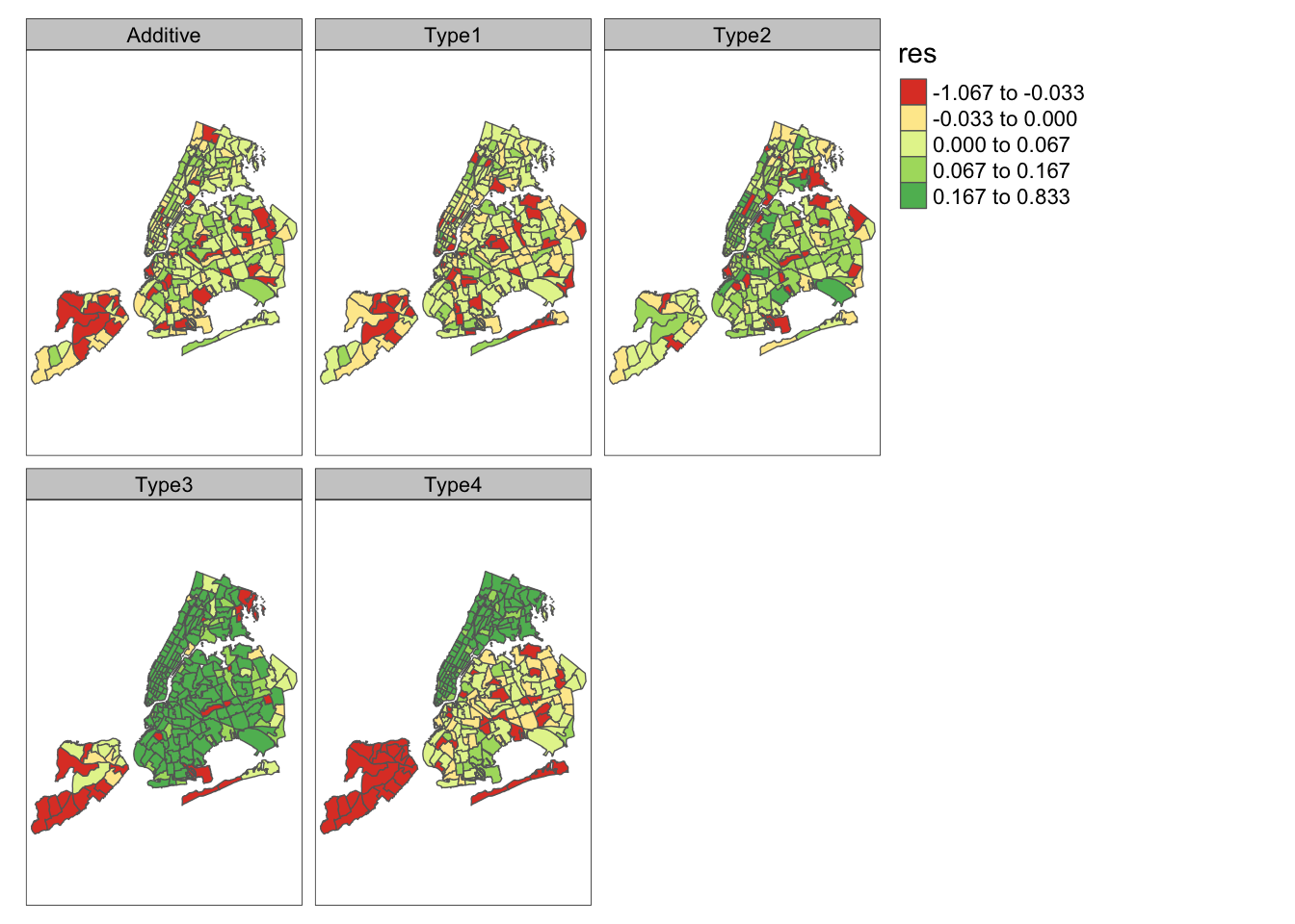

FIGURE 11.1: Time averaged residuals across zones from different models.

Next, we study the behavior of the posterior distributions of \(\nu_i\) and \(\delta_{it}\) under Model KH3. Using inla.posterior.sample(), we generate \(500\) samples from the posterior distributions of \(\nu_i\) and \(\delta_{it}\) from Model KH3. The top panel in Figure 11.2 shows parallel boxplots of the \(\nu_i\) values across \(g=252\) zones, while the bottom panel shows boxplots of time averages of the \(\delta_{it}\) samples. While these boxplots are centered about zero for several zones, we also see non-zero effects in a few taxi zones. The code to obtain the posterior samples is shown below.

post.sampletype3 <-
  inla.posterior.sample(n = 500, tnc.kh3, seed = 1234)
temp.nu <- temp.delta <- list()
for (k in 1:length(post.sampletype3)) {
  x <- post.sampletype3[[k]]
  temp.nu[[k]] <-
    cbind.data.frame(nu = tail(x$latent[grep("id.zone:",
                                             rownames(x$latent))], g),
                     zone = unique(data.kh$zoneid))
  temp.delta[[k]] <-
    cbind.data.frame(delta = x$latent[grep("id.zone.int:",
                                           rownames(x$latent))],
                     zone = data.kh$zoneid) %>%
    group_by(zone) %>%
    summarize(across(delta,  ~ mean(.x)))
}

We can use the code below to construct parallel boxplots for the \(\nu_{i}\) across \(g=252\) zones. The code for the time-averaged \(\delta_{it}\) is similar and is not shown here.

nu.all <- bind_rows(temp.nu)
nu.all$zone <- factor(nu.all$zone, levels = unique(data.kh$zoneid))
p1 <- ggplot(nu.all, aes(x = zone, y = nu)) +
  geom_boxplot(outlier.shape = NA) +
  ylab(expression(nu)) +
  xlab("zone") +
  theme(axis.text.x = element_blank())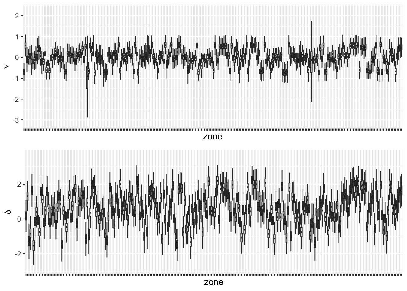

FIGURE 11.2: Boxplots of \(\nu_i\) (top panel) and boxplots of \(\delta_{it}\) averaged over time (bottom panel) for 252 zones.

Figure 11.3 compares the time averaged (over \(n= 30\) months) fitted values from Model KH3 (right plot) with actual monthly TNC usage (left plot) for \(g=252\) zones. The model gives a very close fit.

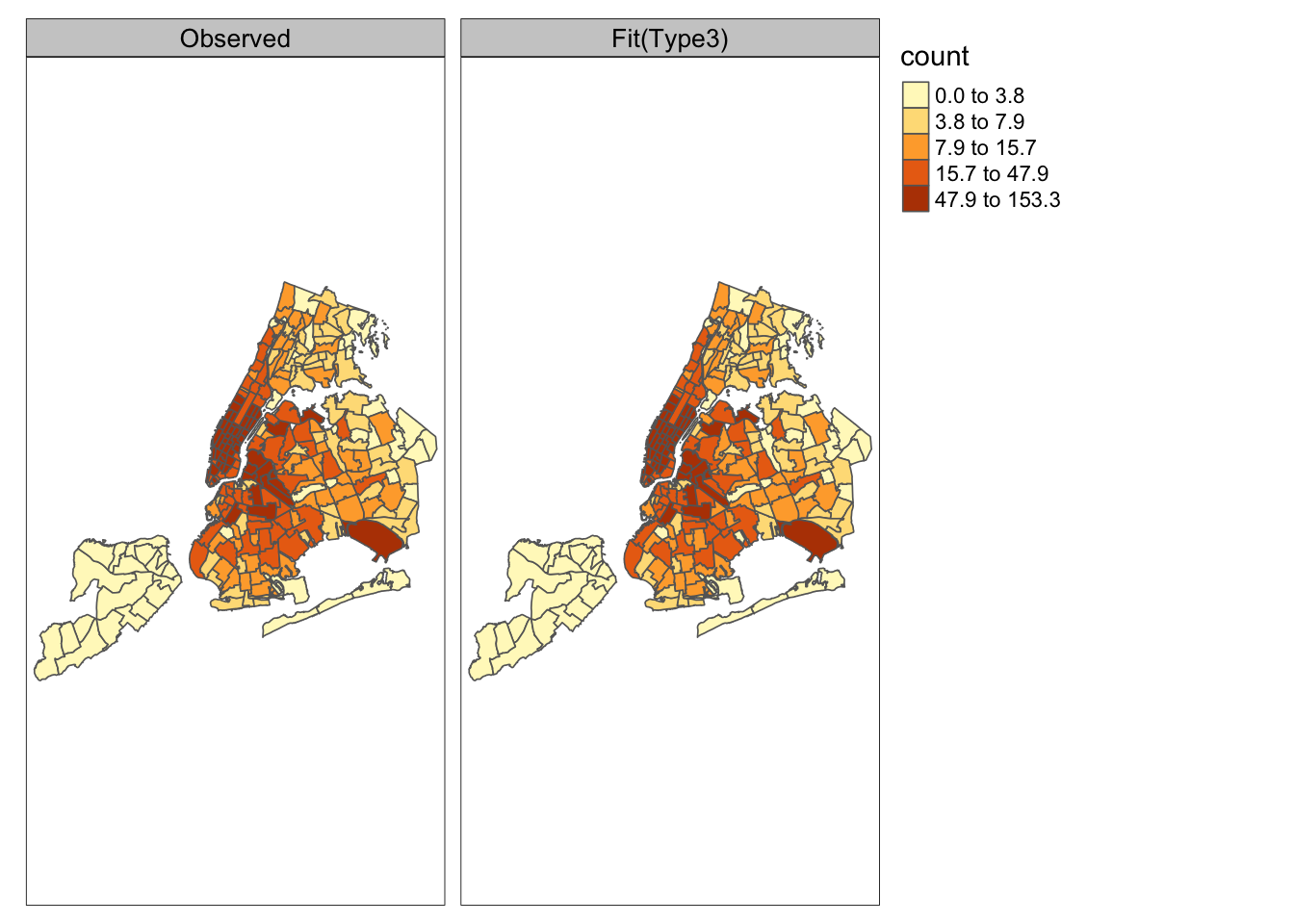
FIGURE 11.3: Observed monthly TNC counts (left) and time averaged fitted counts from Model KH3 (right) for g=252 zones.

References

Bakka, Haakon, Håvard Rue, Geir-Arne Fuglstad, Andrea Riebler, David Bolin, Janine Illian, Elias Krainski, Daniel Simpson, and Finn Lindgren. 2018. “Spatial Modeling with R-INLA: A Review.” Wiley Interdisciplinary Reviews: Computational Statistics 10 (6): e1443.

Besag, Julian. 1974. “Spatial Interaction and the Statistical Analysis of Lattice Systems.” Journal of the Royal Statistical Society: Series B (Methodological) 36 (2): 192–225.

Besag, Julian, Jeremy York, and Annie Mollié. 1991. “Bayesian Image Restoration, with Two Applications in Spatial Statistics.” Annals of the Institute of Statistical Mathematics 43 (1): 1–20.

Blangiardo, Marta, Michela Cameletti, Gianluca Baio, and Håvard Rue. 2013. “Spatial and Spatio-Temporal Models with R-INLA.” Spatial and Spatio-Temporal Epidemiology 4: 33–49.

Cressie, Noel. 2015. Statistics for Spatial Data. New York: John Wiley & Sons.

Fuentes, Montserrat, Li Chen, and Jerry M. Davis. 2008. “A Class of Nonseparable and Nonstationary Spatial Temporal Covariance Functions.” Environmetrics: The Official Journal of the International Environmetrics Society 19 (5): 487–507.

Knorr-Held, Leonhard. 2000. “Bayesian Modelling of Inseparable Space-Time Variation in Disease Risk.” Statistics in Medicine 19 (17-18): 2555–67.

Krainski, Elias T., Virgilio Gómez-Rubio, Haakon Bakka, Amanda Lenzi, Daniela Castro-Camilo, Daniel Simpson, Finn Lindgren, and Håvard Rue. 2018. Advanced Spatial Modeling with Stochastic Partial Differential Equations Using r and INLA. New York: CRC Press.

Lindgren, Finn, and Håvard Rue. 2015. “Bayesian Spatial Modelling with R-INLA.” Journal of Statistical Software 63 (19): 1–25.

Moraga, Paula. 2019. Geospatial Health Data: Modeling and Visualization with r-INLA and Shiny. Boca Raton, Florida: CRC Press.

Van Niekerk, Janet, Haakon Bakka, Håvard Rue, and Loaf Schenk. 2019. “New Frontiers in Bayesian Modeling Using the INLA Package in R.” arXiv Preprint arXiv:1907.10426.

Wikle, Christopher K., Mark L. Berliner, and Noel Cressie. 1998. “Hierarchical Bayesian Space-Time Models.” Environmental and Ecological Statistics 5 (2): 117–54.