Chapter 9 Modeling Count Time Series
9.1 Introduction
This chapter describes use of R-INLA for analyzing time series of counts.
Section 9.2 describes models for a single univariate count time series.
Section 9.3 shows how to fit a dynamic subject-specific model to a set of univariate count time series. To begin, we source the custom functions.
source("functions_custom.R")This chapter uses the following packages.
library(INLA)
library(tidyverse)
We analyze the following data.
Crash counts in CT
Daily bike rentals
Ridesourcing in NYC
9.2 Univariate time series of counts
In the dynamic generalized linear model (DGLM) for a time series of counts, the response variable \(Y_t\) is assumed to have a suitable probability distribution which belongs to the exponential family, negative binomial or Poisson, say. The mean \(E(Y_t) =\mu_t\) is linked to a structured predictor through a link function, \(g(\mu_t) = \log (\mu_t)\). The structured predictor can take the form \(\eta_t = \beta_{t,0} + \sum_{j=1}^k \beta_{t,j} Z_{t,j}\), where \(Z_{t,j},~j=1,\ldots,k\) are exogenous predictors, and the coefficients \(\beta_{t,j},~j=0,\ldots,k\) are regarded as the state parameters in the DGLM, and may evolve randomly as latent Gaussian processes depending on some hyperparameters.
9.2.1 Example: Simulated univariate Poisson counts
We simulate a Poisson time series with mean \(\mu_t\). The observation model and state equation of the DGLM are
\[\begin{align} Y_t \vert \mu_t & \sim \mbox{Poisson}(\mu_t), \notag \\ \log(\mu_t) &= \beta_{t}, \notag \\ \beta_{t} &= \phi \beta_{t-1} + w_{t}, \tag{9.1} \end{align}\] where, \(\beta_{t}\) is an unknown state variable, \(|\phi| < 1\), and \(w_{t}\) is N\((0,\sigma^2_w)\). The count time series corresponding to true values of \(\phi =0.65\) and \(\sigma^2_w =0.25\) is shown in Figure 9.1.
sim.y.ar1.pois <-
  simulation.from.ar.poisson(
    sample.size = 500,
    burn.in = 100,
    phi = 0.65,
    level = 0,
    drift = 0,
    W = 0.25,
    plot.data = TRUE,
    seed = 123457
  )
sim.y.ar1.pois$sim.plot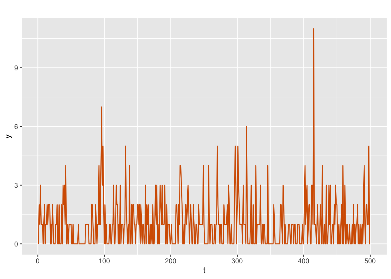
FIGURE 9.1: Time series of simulated Poisson counts.
y.ar1.pois <- sim.y.ar1.pois$sim.data
n <- length(sim.y.ar1.pois$sim.data)
The formula for fitting (9.1) is shown below. Note that in the inla() function, we set the argument control.predictor = list(compute = TRUE, link = 1). The argument compute = TRUE allows the marginals of the linear predictor to be computed. The argument link = 1 specifies the log link corresponding to the Poisson family. Note that, if we do not specify link=1, the identity link would be used by INLA for the hold-out fits, i.e., \(\eta_t\) will be linked to \(\mu_t\) instead of \(\log(\mu_t)\). The results from the posterior distributions of the hyperparameters \(\phi\) and \(\sigma^2_w\) show that we are able to recover the true values in the simulation.
id <- 1:n
sim.pois.dat <- cbind.data.frame(y.ar1.pois, id)
formula <- y.ar1.pois ~ f(id, model = "ar1") - 1
model.sim.pois <- inla(
  formula,
  family = "poisson",
  data = sim.pois.dat,
  control.predictor = list(compute = TRUE, link = 1)
)
#summary(model.sim.pois)
format.inla.out(model.sim.pois$summary.hyperpar[,c(1:2)])
##   name             mean  sd
## 1 Precision for id 3.137 0.755
## 2 Rho for id       0.590 0.124
We first use inla.tmarginal to obtain the marginal distribution of the state variance, and then
compute its 95% HPD interval using inla.hpdmarginal() as shown below.
state.var <-  inla.tmarginal(
  fun = function(x)
    exp(-x),
  marginal =
    model.sim.pois$internal.marginals.hyperpar$`Log precision for id`
)
var.state.hpd.interval <- inla.hpdmarginal(p = 0.95, state.var)
round(var.state.hpd.interval, 3)
##              low  high
## level:0.95 0.193 0.492
In the code below, summary.fitted.values returns summaries of the posterior marginals of the fitted values which are obtained by transforming the linear predictors by the inverse of the link function.
head(model.sim.pois$summary.fitted.values$mean) %>%
  round(3)
## [1] 1.012 1.293 1.318 1.582 1.255 1.123
However, note that these cannot be obtained by directly applying the inverse transformation to summary.linear.predictor, which returns summaries of posterior marginals of the linear predictors in the model.. For example, under a log link, we cannot just apply the exp() function to summary.linear.predictor$mean, since this will not result in summary.fitted.values$mean.
exp(head(model.sim.pois$summary.linear.predictor$mean)) %>%
  round(3)
## [1] 0.906 1.173 1.200 1.444 1.142 1.018
We must instead transform the marginals for the variable fitted.from.lp.
fitted.from.lp <- model.sim.pois$marginals.linear.predictor %>%
  sapply(function(x)
    inla.emarginal(
      fun = function(y)
        exp(y),
      marginal = x
    ))
head(fitted.from.lp) %>%
  round(3)
## Predictor.1 Predictor.2 Predictor.3 Predictor.4 Predictor.5
##       1.012       1.293       1.318       1.582       1.255
## Predictor.6
##       1.122
Fitted values, i.e., means of the posterior predictive distributions (blue), along with the interval between the \(2.5^{th}\) and \(97.5^{th}\) percentiles (gray shaded region), are shown in Figure 9.2.
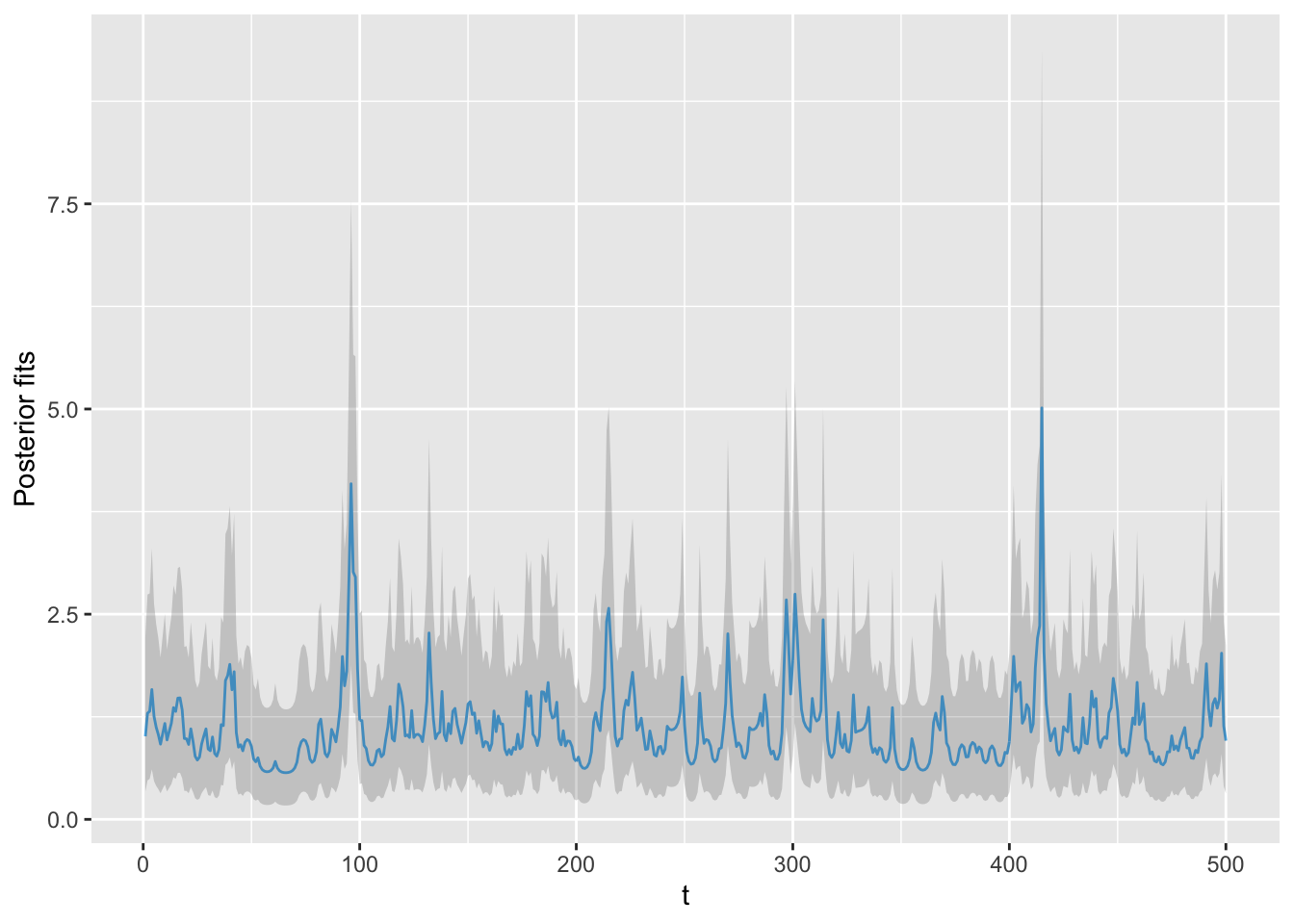
FIGURE 9.2: Means of the posterior predictive distributions (blue) and the interval between the \(2.5^{th}\) and \(97.5^{th}\) percentiles (gray shaded region).
9.2.2 Example: Modeling crash counts in CT
Hu et al. (2013) described a DGLM in the context of transportation safety. The data7 is obtained from records for all crashes on state-maintained roads in Connecticut from January 1995 to December 2009 collected from the Connecticut Department of Transportation (ConnDOT). Crashes are grouped by level of severity, which include fatal (K), severe injury (A), evident minor injury (B), non-evident possible injury (C), and property damage only (O). For each month, crash counts are aggregated at each severity level by access type (surface or limited access roads), area type (rural or urban), and whether or not the driver of at least one of the vehicles involved in the crash was a senior. Severity for a crash is defined as the highest injury severity experienced by any individual involved. Monthly average daily vehicle miles traveled (VMT) in each of these four categories are obtained by applying monthly expansion factors (obtained from ConnDOT) to annual average daily VMTs (see Hu et al. (2013) for details). We model a univariate time series of monthly KAB crash counts, by cumulating crashes of type K, A, or B that involved senior drivers and occurred on rural, limited access roads. The predictor is the VMT, denoted here by \(V_t\). We use a negative binomial DGLM with \(\mu_t = E(Y_t)\), and shape parameter \(\kappa\). The observation model of the DGLM is
\[\begin{align} Y_t \vert \mu_t & \sim \mbox{NegBin}(\mu_t,k), \text{ where}, \notag \\ \mu_t & = \alpha_t V_t^{\beta_{t,1}}, \text{ i.e.}, \notag \\ \log(\mu_t) & = \beta_{t,0} + \beta_{t,1} Z_t, \tag{9.2} \end{align}\] where \(\beta_{t,0}= \log(\alpha_t)\) and \(Z_t = \log(V_t)\). Let \(\boldsymbol{\beta}_{t}=(\beta_{t,0},\beta_{t,1})'\) be a 2-dimensional state (parameter) vector, which evolves according to the state equations shown below:
\[\begin{align} \beta_{t,0} &= \beta_{t-1,0} + w_{t,0}, \notag \\ \beta_{t,1} &= \beta_{t-1,1} + w_{t,1}, \tag{9.3} \end{align}\] where \(w_{t,0} \sim N(0, W_0)\) and \(w_{t,1} \sim N(0, W_1)\). The time series is shown in Figure 9.3.
dat <-
  read.csv(file = "crashcount_rle.csv",
           header = TRUE,
           stringsAsFactors = FALSE)
n <- nrow(dat)
kabct <- dat$KAB_FREQ
vmt <-  log(dat$vmt_exp)
tsline(kabct,
        xlab = "t",
        ylab = "crash counts",
        line.color = "red", line.size = 0.6)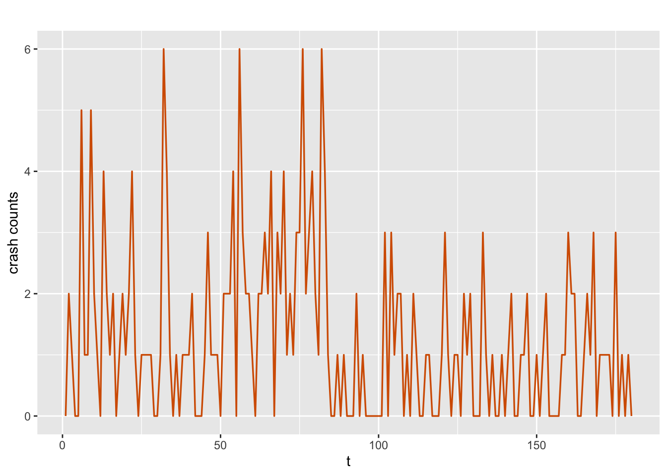
FIGURE 9.3: Time series of crash counts.
The indexes, data frame, and formula are as follows.
id.b0 <- id.b1 <- 1:n
data.crash <- data.frame(id.b0, id.b1, kabct, vmt)
formula.crashct <-
  kabct ~  -1 + f(id.b0,
             model = "rw1",
             initial = 5,
             constr = FALSE) +
  f(id.b1,
    vmt,
    model = "rw1",
    initial = 5,
    constr = FALSE)
A summary of the results is shown below. The plots in Figure 9.4 show the posterior means of the state variables, i.e., the dynamic intercept on the log scale (\(\beta_{t,0}\)), and the dynamic slope \(\beta_{t,1}\).
model.crashct = inla(
  formula.crashct,
  family = "nbinomial",
  data = data.crash,
  control.compute = list(
    dic = TRUE,
    waic = TRUE,
    cpo = TRUE,
    config = TRUE
  ),
  control.family = list(hyper = list(theta = list(
    prior = "loggamma",
    param = c(1, 1)
  )))
)
#summary(model.crashct)
format.inla.out(model.crashct$summary.hyperpar[, c(1:2)])
##   name                                    mean      sd
## 1 size for nbinomial obs 1/overdispersion     2.942     0.974
## 2 Precision for id.b0                     19671.628 21737.167
## 3 Precision for id.b1                     13947.980 41998.126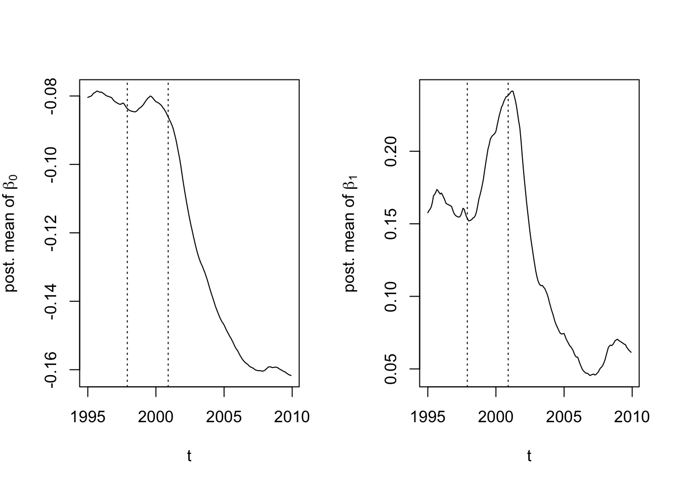
FIGURE 9.4: Posterior means of intercepts on the log scale (left) and the slope (right).
The vertical dotted lines in Figure 9.4 correspond to September 1997 and September 2000, when stricter passenger car regulation standards were implemented for airbags and anti-lock brakes, respectively. It is interesting to see how the estimated posterior means of \(\beta_{t,0}\) and \(\beta_{t,1}\) behave over time, and how they respond to the two events. We see that on rural limited access roads, senior drivers show a decreasing trend in the posterior mean of \(\beta_{t,0}\) after the second intervention, and decreasing pattern in the posterior mean of \(\beta_{t,1}\), with a bump at the end. Overall, there are interesting temporal patterns for the KAB injury crashes on these selected roads.
A static negative binomial loglinear model (code shown below) can be compared with the DGLM fit; we do not show these results here, but they are available in the GitHub link for the book.
reg.negbin <- MASS::glm.nb(kabct ~ vmt, link = log)
summary(reg.negbin)
9.2.3 Example: Daily bike rentals in Washington D.C.
We use data on daily bike sharing customers and weather in the metro DC area from January 1, 2011 to December 31, 2018. The data is obtained from Kaggle.8
We model the daily bike usage as a function of temperature (Fahrenheit), humidity, and wind speed. We set aside the last \(n_h = 7\) data points for validating the model fit.
bike <- read.csv("bikeusage_daily.csv")
n <- nrow(bike)
n.hold <- 7
n.train <- n - n.hold
test.data <- tail(bike$Total.Users, n.hold)
train.data <- bike[1:n.train, ]
The time series (see Figure 9.5) exhibits periodic behavior, with period \(s=7\). We set up a model with trend and seasonality (with period \(s=7\)), and the weather variables as predictors.
n.seas <- s <-  7
y <- train.data$Total.Users
y.append <- c(y, rep(NA, n.hold))
id <- id.trend <-  id.seas <- 1:length(y.append)
bike.dat <-
  cbind.data.frame(id,
                   id.trend,
                   id.seas,
                   y.append,
                   select(bike, Temperature.F:Wind.Speed))
We fit a Poisson DGLM, treating only the trend and seasonal effects as random (similar to the structural time series model in Chapter 5), while the weather effects are treated as fixed effects. The observation model is
\[\begin{align} Y_t \vert \mu_t & \sim \mbox{Poisson}(\mu_t), \notag \\ \log(\mu_t) &= m_t + S_t + \boldsymbol{z}'_t \boldsymbol{\beta}, \tag{9.4} \end{align}\] where \(m_t\) and \(S_t\) are the random trend and seasonal effects modeled as shown below, and \(\boldsymbol{\beta}\) is a vector of static coefficients corresponding to the exogenous predictors \(\boldsymbol{z}_t\). We model the latent state variables by
\[\begin{align} m_{t} &= m_{t-1} + w_{t,1}, \nonumber \\ S_t & = -\sum_{j=1}^6 S_{t-j} + w_{t,2}, \tag{9.5} \end{align}\] where \(w_{t,j} \sim N(0,\sigma^2_{w_j}),~j=1,2\). The formula and fit are shown below.
bike.formula <- y.append ~  Temperature.F + Humidity + Wind.Speed +
  f(id.trend, model = "rw1") +
  f(id.seas, model = "seasonal", season.length = n.seas)
bike.model <- inla(
  bike.formula,
  family = "poisson",
  data = bike.dat,
  control.predictor = list(compute = TRUE, link = 1),
  control.compute = list(
    dic = TRUE,
    waic = TRUE,
    cpo = TRUE,
    config = TRUE
  ),
  control.family = list(link = "log")
)
#summary(bike.model)
format.inla.out(bike.model$summary.fixed[,c(1:5)])
##   name          mean   sd    0.025q 0.5q   0.975q
## 1 Intercept      5.035 0.129  4.782  5.035  5.287
## 2 Temperature.F  0.015 0.002  0.012  0.015  0.019
## 3 Humidity      -0.011 0.001 -0.012 -0.011 -0.009
## 4 Wind.Speed    -0.004 0.001 -0.007 -0.004 -0.002
format.inla.out(bike.model$summary.hyperpar[,c(1:2)])
##   name                   mean  sd
## 1 Precision for id.trend 24.33 4.253
## 2 Precision for id.seas  44.73 8.381
Using the approach described in Section 9.2.1, we obtain fitted values using summary.fitted.values$mean. These are plotted in Figure 9.5.
fit.bike <- bike.model$summary.fitted.values$mean
fit.bike.df <-
  cbind.data.frame(
    time = 1:n,
    obs.bike = bike$Total.Users,
    fit.bike = fit.bike
  )
multiline.plot(
  fit.bike.df,
  line.size = 0.5,
  xlab = "t",
  ylab = "bike counts",
  line.color = c("red", "blue")
)+
  theme(legend.position = "none")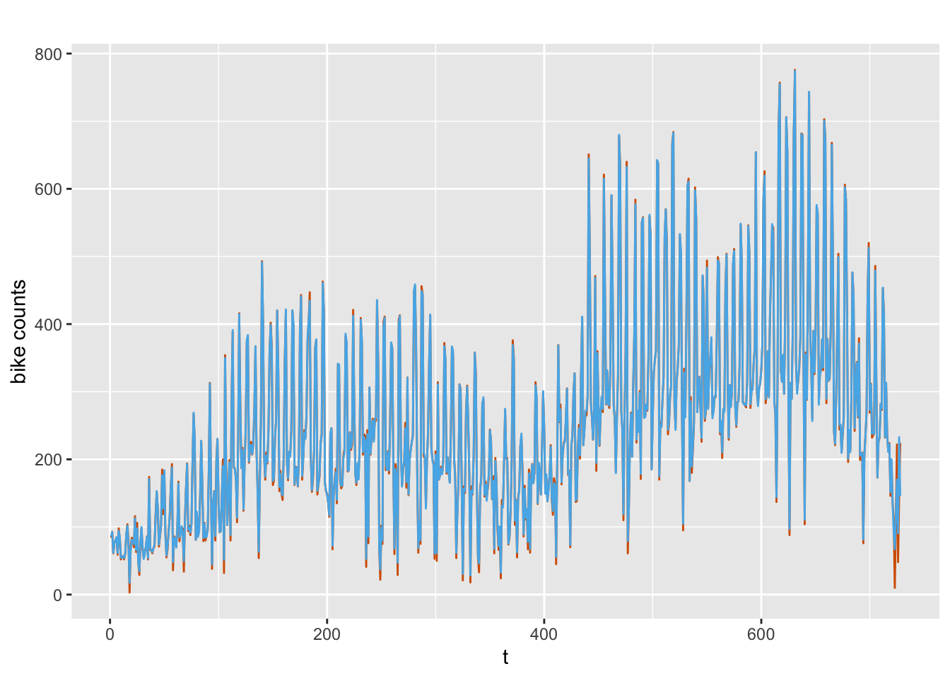
FIGURE 9.5: Observed (red) and fitted (blue) bike counts.
We compute out-of-sample forecasts of the hold-out data, and then compute the MAE.
yfore <- tail(fit.bike, n.hold)
mae(test.data, round(yfore))
## [1] "MAE is 50.143"
Note that we can fit other models to this data by (a) selecting the best subset of exogenous predictors, (b) replacing the random walk evolution for \(m_t\) by other processes, or (c) replacing the Poisson sampling distribution for \(Y_t\) by the negative binomial distribution. We can compare the different models for bike usage using criteria such as the DIC, WAIC, and MAE.
9.3 Hierarchical modeling of univariate count time series
This section describes fitting a hierarchical (subject-specific) dynamic model to a set of \(g\) time series of counts, each of length \(n\). In Section 9.3.1, we present the code and results for three scenarios used to model several univariate time series of counts. In Section 9.3.2, we illustrate such models for daily TNC counts over three years for taxi zones in Manhattan (see Section 6.3).
9.3.1 Example: Simulated univariate Poisson counts
Let \(y_{it}\) denote the counts at time \(t\) from the \(i\)th series, for \(t=1,\ldots,n\) and \(i=1,\ldots,g\). Let \(E(y_{it}) = \lambda_{it}\). For simplicity, we first assume that there are no exogenous predictors, and build the following model:
\[\begin{align} y_{it}|\lambda_{it} &\sim \mbox{UDC}(\lambda_{it}), \notag \\ \log \lambda_{it} &= \alpha_i + \beta_{it,0}, \notag \\ \beta_{it,0} &= \phi \beta_{i,t-1,0}+ w_{it}, \tag{9.6} \end{align}\] where, we assume that UDC refers to univariate distribution of counts, such as the Poisson, negative binomial, or zero-inflated Poisson (ZIP) distributions. We allow the intercept \(\beta_{it,0}\) to be random, varying over \(i\) and \(t\), evolving over time as an AR(1) process. We assume that \(w_{it}\) are N\((0, \sigma^2_w)\) variables, and UDC refers to the Poisson distribution. We discuss three separate cases, based on our assumption about the level.
Case 1. Common level model
We allow the \(g=300\) series to have the same level \(\alpha\), i.e., \(\alpha_i =\alpha\) in (9.6). In the simulation, we allow the AR coefficient \(\phi\) to vary slightly around a true value of \(0.8\) across the \(g\) series, and let \(\alpha =1.3\).
set.seed(123457)
g <- 300
n <- 100
burn.in <- 500
n.tot <- n + burn.in
sigma2.w <- 0.25
phi.0 <- 0.8
alpha <- 1.3
yit.all <- yit.all.list <- z1.all <- z2.all <- vector("list", g)
for (j in 1:g) {
  yit <- beta.0t <- lambda.t <- eta.t <- vector("double", n.tot)
  u <- runif(1, min = -0.1, max = 0.05)
  phi <- phi.0 + u
  beta.0t <-
    arima.sim(list(ar = phi, ma = 0), n = n.tot, sd = sqrt(sigma2.w))
  for (i in 1:n.tot) {
    eta.t[i] <- alpha + beta.0t[i]
    lambda.t[i] <- exp(eta.t[i])
    yit[i] <- rpois(1, lambda.t[i])
  }
  yit.all.list[[j]] <- tail(yit, n)
}
yit.all <- unlist(yit.all.list)
We set up indexes, data frame, and formula, and fit the common level model.
id.beta0 <- rep(1:n, g)
re.beta0 <- rep(1:g, each = n)
data.hpois.alpha.1 <-
  cbind.data.frame(id.beta0, yit.all, re.beta0)
formula.hpois.alpha.1 <-
yit.all ~ 1 + f(id.beta0, model = "ar1", replicate = re.beta0)model.hpois.alpha.1 <- inla(
formula.hpois.alpha.1,
family = "poisson",
data = data.hpois.alpha.1,
control.predictor = list(compute = TRUE, link = 1),
control.compute = list(
dic = TRUE,
cpo = TRUE,
waic = TRUE,
config = TRUE,
cpo = TRUE
)
)The results for the fixed and random parameters are shown below. We see that all the true parameters in the simulation are adequately recovered.
format.inla.out(summary.hpois.alpha.1$fixed)[c(1:5)]
##   name      mean  sd    0.025q 0.5q  0.975q mode  kld
## 1 Intercept 1.294 0.013 1.268  1.294 1.32   1.294 0
##        name  mean    sd 0.025q  0.5q
## 1 Intercept 1.294 0.013  1.268 1.294
format.inla.out(summary.hpois.alpha.1$hyperpar[c(1,2,4,5)])
##   name                   mean  sd    0.5q  0.975q
## 1 Precision for id.beta0 1.581 0.031 1.583 1.638
## 2 Rho for id.beta0       0.780 0.005 0.780 0.789
Alternatively, we can fit the model under the following non-default prior specification,
prior.hpois <- list(
   prec = list(prior = "loggamma", param = c(0.1, 0.1)),
   rho = list(prior = "normal", param = c(0, 0.15))
 )
and then modify the following line of code in the formula as
formula.hpois.alpha.1.nd.prior <-
  yit.all ~ 1 + f(id.beta0,
                  model = "ar1",
                  replicate = re.beta0,
                  hyper = prior.hpois)
Results are available on our GitHub link.
Case 2. Model with different fixed levels
We simulate data from the model (9.6) with different fixed levels \(\alpha_i,~i=1,\ldots,g\), for \(g=10\). We allow the coefficient of an exogenous predictor \(Z_{it}\) to evolve dynamically as an AR(1) model with coefficient \(\phi=0.8\) and \(\sigma^2_w = 0.25\).
set.seed(123457)
g <- 10
n <- 100
burn.in <- 500
n.tot <- n + burn.in
sigma2.w0 <- 0.25
phi.0 <- 0.8
We slightly perturb the values of \(\phi\) and \(\sigma^2_w\)
to reflect variability that would occur in practice.
We use arima.sim() to generate underlying AR(1) models for the latent states and build the responses and predictors.
yit.all <-
  yit.all.list <-
  z1.all <- z2.all <- alpha <- z.all <- sigma2.w <- vector("list", g)
for (j in 1:g) {
  yit <- beta.1t <- lambda.t <- eta.t <- z <- vector("double", n.tot)
  u <- runif(1, min = -0.1, max = 0.05)
  phi <- phi.0 + u
  us <- runif(1, min = -0.15, max = 0.25)
  sigma2.w[[j]] <- sigma2.w0 + us
  beta.1t <-
    arima.sim(list(ar = phi, ma = 0), n = n.tot, sd = sqrt(sigma2.w[[j]]))
  alpha[[j]] <- sample(seq(-2, 2, by = 0.1), 1)
  z <- rnorm(n.tot)
  for (i in 1:n.tot) {
    eta.t[i] <- alpha[[j]] + beta.1t[i]  * z[i]
    lambda.t[i] <- exp(eta.t[i])
    yit[i] <- rpois(1, lambda.t[i])
  }
  yit.all.list[[j]] <- tail(yit, n)
  z.all[[j]] <- tail(z, n)
}
yit.all <- unlist(yit.all.list)
z.all <- unlist(z.all)
alpha.all <- unlist(alpha)
The indexes, replicates, and formula are set up as shown below. The fixed \(\alpha_i\)’s are handled by
fact.alpha <- as.factor(id.alpha).
id.beta1 <- rep(1:n, g)
re.beta1 <- id.alpha <- rep(1:g, each = n)
fact.alpha <- as.factor(id.alpha)
formula.hpois.alpha.2 <-
  yit.all ~ -1 + fact.alpha +
  f(id.beta1, z.all, model = "ar1", replicate = re.beta1)
data.hpois.alpha.2 <-
  cbind.data.frame(id.beta1, z.all, yit.all, re.beta1, fact.alpha)
The inla() call for model.hpois.alpha.2 is similar to the code for model.hpois.alpha.1, except for the replaced inputs formula.hpois.alpha.2 and data.hpois.alpha.2. They produce the results shown below.
format.inla.out(summary.hpois.alpha.2$fixed)[c(1:5)]
##    name         mean   sd    0.025q 0.5q   0.975q mode   kld
## 1  fact.alpha1  -2.530 0.328 -3.225 -2.513 -1.933 -2.478 0
## 2  fact.alpha2  -1.882 0.250 -2.403 -1.872 -1.421 -1.851 0
## 3  fact.alpha3  -1.917 0.248 -2.432 -1.907 -1.458 -1.887 0
## 4  fact.alpha4  -0.613 0.145 -0.908 -0.610 -0.338 -0.603 0
## 5  fact.alpha5  -1.182 0.180 -1.551 -1.177 -0.845 -1.165 0
## 6  fact.alpha6   1.425 0.060  1.306  1.426  1.541  1.427 0
## 7  fact.alpha7  -1.025 0.170 -1.374 -1.020 -0.706 -1.010 0
## 8  fact.alpha8   0.043 0.111 -0.181  0.045  0.255  0.050 0
## 9  fact.alpha9   1.285 0.063  1.160  1.286  1.406  1.287 0
## 10 fact.alpha10 -0.693 0.150 -0.998 -0.689 -0.410 -0.682 0
##            name   mean    sd 0.025q   0.5q
## 1   fact.alpha1 -2.530 0.328 -3.225 -2.513
## 2   fact.alpha2 -1.882 0.250 -2.403 -1.872
## 3   fact.alpha3 -1.917 0.248 -2.432 -1.907
## 4   fact.alpha4 -0.613 0.145 -0.908 -0.610
## 5   fact.alpha5 -1.182 0.180 -1.551 -1.177
## 6   fact.alpha6  1.425 0.060  1.306  1.426
## 7   fact.alpha7 -1.025 0.170 -1.374 -1.020
## 8   fact.alpha8  0.043 0.111 -0.181  0.045
## 9   fact.alpha9  1.285 0.063  1.160  1.286
## 10 fact.alpha10 -0.693 0.150 -0.998 -0.689
format.inla.out(summary.hpois.alpha.2$hyperpar[c(1,2,4,5)])
##   name                   mean  sd    0.5q  0.975q
## 1 Precision for id.beta1 1.836 0.296 1.813 2.482
## 2 Rho for id.beta1       0.824 0.043 0.828 0.896
The estimated \(\alpha_i\)’s recover the true levels shown below:
alpha.all
##  [1] -1.8 -1.6 -2.0 -0.8 -1.1  1.4 -1.2  0.0  1.3 -0.9
Case 3. Model with different random levels
Let \(\alpha_i\)’s be independent N\((0,\sigma^2_\alpha)\) random variables, an assumption which is particularly useful when \(g\) is large, and we are only interested in investigating whether there is significant variation in the large population of time series from which \(g\) series are randomly drawn. The true parameters are the similar to Case 2, but \(g=500\) instead of \(10\). We set
alpha[[j]] <- sample(seq(-2, 2, by = 0.1), 1) and generate the responses and predictors.
yit.all <-
  yit.all.list <-
  z1.all <- z2.all <- alpha <- z.all <- sigma2.w <- vector("list", g)
for (j in 1:g) {
  yit <- beta.1t <- lambda.t <- eta.t <- z <- vector("double", n.tot)
  u <- runif(1, min = -0.1, max = 0.05)
  phi <- phi.0 + u
  us <- runif(1, min = -0.15, max = 0.25)
  sigma2.w[[j]] <- sigma2.w0 + us
  beta.1t <-
    arima.sim(list(ar = phi, ma = 0), n = n.tot, sd = sqrt(sigma2.w[[j]]))
  alpha[[j]] <- sample(seq(-2, 2, by = 0.1), 1)
  z <- rnorm(n.tot)
  for (i in 1:n.tot) {
    eta.t[i] <- alpha[[j]] + beta.1t[i]  * z[i]
    lambda.t[i] <- exp(eta.t[i])
    yit[i] <- rpois(1, lambda.t[i])
  }
  yit.all.list[[j]] <- tail(yit, n)
  z.all[[j]] <- tail(z, n)
}
yit.all <- unlist(yit.all.list)
z.all <- unlist(z.all)
Unlike Case 2, we set id.alpha <- rep(1:g, each = n) and include it as a random effect in the formula. The inla() call is similar to Case 2 except for replacing that formula and data frame by formula.hpois.alpha.3 and
data.hpois.alpha.3. The results are shown below.
id.beta1 <- rep(1:n, g)
re.beta1 <- id.alpha <- rep(1:g, each = n)
prec.prior <- list(prec = list(param = c(0.001, 0.001)))
formula.hpois.alpha.3 <-
  yit.all ~ -1 + f(id.alpha, model="iid") +
  f(id.beta1, z.all, model = "ar1", replicate = re.beta1)
data.hpois.alpha.3 <-
cbind.data.frame(id.beta1, z.all, yit.all, re.beta1, id.alpha)format.inla.out(summary.hpois.alpha.3$hyperpar[c(1,2,4,5)])
## name mean sd 0.5q 0.975q
## 1 Precision for id.alpha 0.703 0.064 0.693 0.853
## 2 Precision for id.beta1 1.311 0.026 1.309 1.368
## 3 Rho for id.beta1 0.780 0.005 0.780 0.790Similar to Case 2, we are able to recover the true \(\phi\) and \(\sigma^2\). The estimated posterior precision matches the true precision of the simulated random \(\alpha\)’s. The estimation accuracy will increase as \(g\) increases.
9.3.2 Example: Modeling daily TNC usage in NYC
We fit hierarchical count data models to TNC usage in the borough of Manhattan in NYC, consisting of 36 taxi zones. The variables are similar to what we have seen in Chapter 6 for weekly ridesourcing data. In almost every taxi zone in Manhattan, TNC usage shows an upward trend, Taxi usage shows a slight negative trend, while Subway usage seems relatively flat. Further, both TNC and Taxi usage exhibit periodicity, with seasonal period \(s=7\).
ride.3yr <-
  read.csv("tnc_daily_data.csv",
           header = TRUE,
           stringsAsFactors = FALSE)
ride <- ride.3yr
ride <- ride %>%
  filter(borough == "Manhattan")
n <- n_distinct(ride$date)
g <- n_distinct(ride$zoneid)
uid <- unique(ride$zoneid) #36 zones
ride.zone <- ride
Figure 9.6 shows scaled TNC and Taxi usage for the first nine zones.
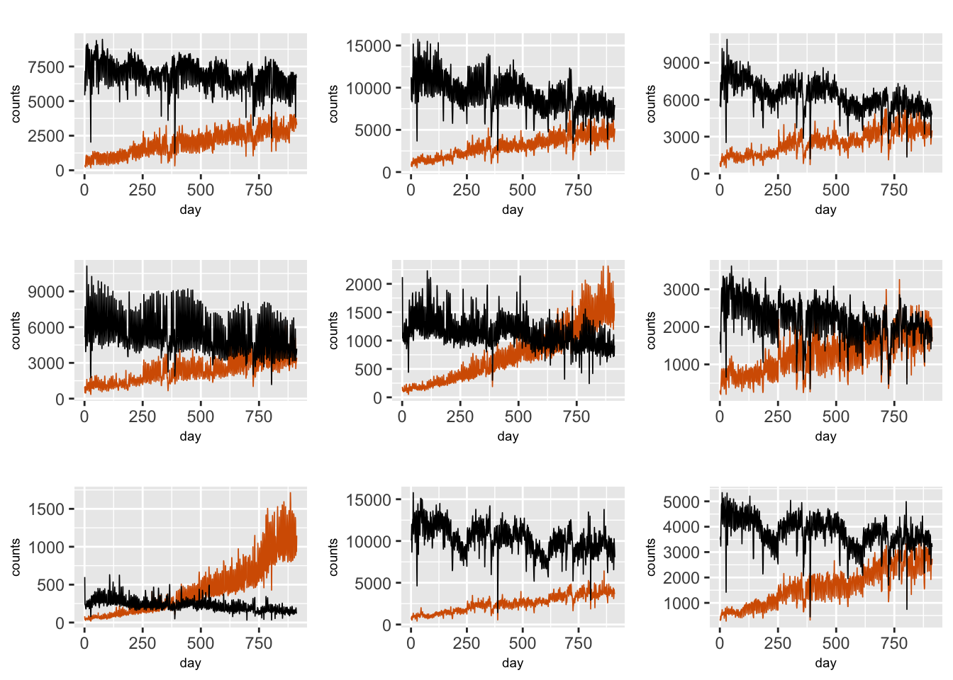
FIGURE 9.6: Time series plots of daily TNC (red) and Taxi (black) counts in nine different taxi zones in Manhattan.
To understand the behavior of daily TNC counts over the three years, we first investigate separate DLM fits to the data from each of the 36 zones. For simplicity, we have suppressed the subscript \(i\) in the individual zone models below. In a given zone, we let \(y_{t}\) denote the daily TNC usage on day \(t\) with \(E(y_{t}) = \lambda_{t}\), and let UDC denote the Poisson distribution. We investigate three different separate zone models, Models Z1–Z3, which capture the time evolution in different ways.
Model Z1
Model Z1 includes a fixed level \(\alpha\), a fixed linear trend \(\gamma t\), a random dynamic intercept \(\beta_{t,0}\) which is modeled as a random walk process, effects of predictors \(\cos(2 \pi t/7)\) and \(\sin(2 \pi t/7)\) to handle the seasonality, and effects of Taxi and Subway usage as fixed predictors. We denote these fixed predictors by \(Z_{t,j},~j=1,\ldots,4\).
\[\begin{align} y_{t}|\lambda_{t} &\sim \mbox{Poisson}(\lambda_{t}), \notag \\ \log \lambda_{t} &= \alpha + \beta_{t,0} + \gamma t + \sum_{j=1}^4 \beta_j Z_{t,j} \notag \\ \beta_{t,0} &= \beta_{t-1,0}+ w_{t,0}, \tag{9.7} \end{align}\] where \(w_{t,0}\) is N\((0, \sigma^2_{w0})\). We set up the indexes and arrays for collecting output from the different zones.
id.t <- 1:n
trend <- 1:n
seas.per <- 7
costerm <- cos(2*pi*trend/seas.per)
sinterm <- sin(2*pi*trend/seas.per)
corr.zone <- vector("list", g)
prec.int <-  vector("list", g)
alpha.coef  <-  taxi.coef <- subway.coef <- vector("list", g)
trend.coef <- cos.coef <- sin.coef <- vector("list", g)
dic.zone <- waic.zone <- mae.zone <- vector("list",g)
We next loop across the \(g\) zones, fitting Model Z1 in each zone, and saving the results. Note that we also investigate the correlation between the stationary time series of model residuals for TNC and Taxi after detrending and deseasonalizing both series.
for (k in 1:g) {
  ride.temp <- ride.zone[ride.zone$zoneid == uid[k], ]
  ride.temp$tnc <- round(ride.temp$tnc / 100)
  ride.temp$taxi <- round(ride.temp$taxi / 100)
  ride.temp$subway <- round(ride.temp$subway / 1000)
  zone.dat <-
    cbind.data.frame(ride.temp, trend, costerm, sinterm, id.t)
  lm.fit.tnc <-
    lm(ride.temp$tnc ~ trend + costerm + sinterm, data = zone.dat)
  res.tnc <- lm.fit.tnc$resid
  lm.fit.taxi <- lm(ride.temp$taxi ~ trend + sin(2 * pi * trend / 7) +
                      cos(2 * pi * trend / 7),
                    data = zone.dat)
  res.taxi <- lm.fit.taxi$resid
  corr.zone[[k]] <- cor(res.tnc, res.taxi)
  #ccf(res.tnc, res.taxi)
  formula.zone.Z1 <-
    tnc ~ 1 + trend + costerm + sinterm + taxi + subway +
    f(id.t, model = "rw1", constr = FALSE)
  model.zone.Z1 <- inla(
    formula.zone.Z1,
    family = "poisson",
    data = zone.dat,
    control.predictor = list(compute = TRUE, link = 1),
    control.compute = list(
      dic = TRUE,
      cpo = TRUE,
      waic = TRUE,
      config = TRUE,
      cpo = TRUE
    )
  )
  prec.int[[k]] <- model.zone.Z1$summary.hyperpar$mean[1]
  alpha.coef[[k]] <- model.zone.Z1$summary.fixed$mean[1]
  trend.coef[[k]] <- model.zone.Z1$summary.fixed$mean[2]
  cos.coef[[k]] <- model.zone.Z1$summary.fixed$mean[3]
  sin.coef[[k]] <- model.zone.Z1$summary.fixed$mean[4]
  taxi.coef[[k]] <- model.zone.Z1$summary.fixed$mean[5]
  subway.coef[[k]] <- model.zone.Z1$summary.fixed$mean[6]
  dic.zone[[k]] <- model.zone.Z1$dic$dic
  waic.zone[[k]] <- model.zone.Z1$waic$waic
  fit.zone <- model.zone.Z1$summary.fitted.values$mean
  mae.zone[[k]] <- sum(abs(ride.temp$tnc - fit.zone)) / n
}
To see the results, we unlist the saved output from all \(g\) zones. There is moderate contemporaneous correlation between TNC and Taxi usage (after detrending and deseasonalizing to make each series more or less stationary); see Figure 9.7. The ccf() plots (not shown) do not show much evidence that Taxi usage dynamically drives TNC usage. This is reflected in Models Z1–Z3 by not including a dynamic evolution for its coefficient, \(\beta_3\).
model.zone.Z1.result <-
  list(
    corr.zone = unlist(corr.zone),
    prec.int = unlist(prec.int),
    alpha.coef = unlist(alpha.coef),
    trend.coef = unlist(trend.coef),
    cos.coef = unlist(cos.coef),
    sin.coef = unlist(sin.coef),
    taxi.coef = unlist(taxi.coef),
    subway.coef = unlist(subway.coef),
    dic.zone = unlist(dic.zone),
    waic.zone = unlist(waic.zone),
    mae.zone = unlist(mae.zone)
  )
out.corr <- model.zone.Z1.result$corr.zone
summary(out.corr)
## Min. 1st Qu. Median Mean 3rd Qu. Max.
## 0.111 0.453 0.594 0.525 0.638 0.752
hist(out.corr, main = "", xlab="correlation", ylab="")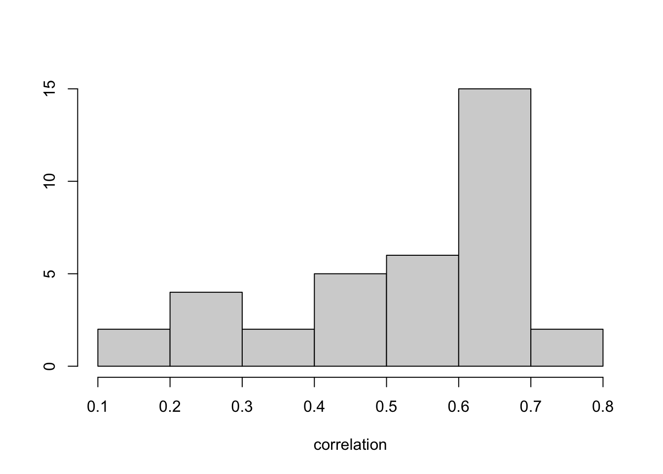
FIGURE 9.7: Histogram of correlations between residuals of TNC and Taxi usage after fitting Model Z1 across taxi zones.
Histograms of the estimated coefficients from the \(g\) zones (see Figure 9.8) can be used to investigate whether the zones exhibit relatively homogeneous behavior, or whether there are outlying zones, say. Histograms of DIC, WAIC, and MAE are shown in Figure 9.9. These can be used to compare Model Z1 to Models Z2–Z3 (see below).
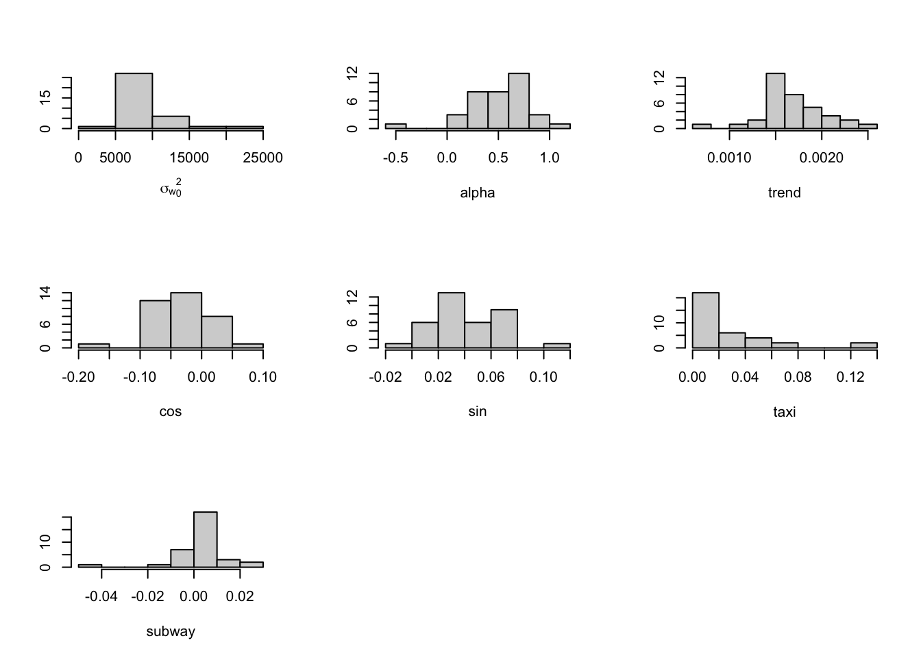
FIGURE 9.8: Histograms of the estimated coefficients from Model Z1 across taxi zones.
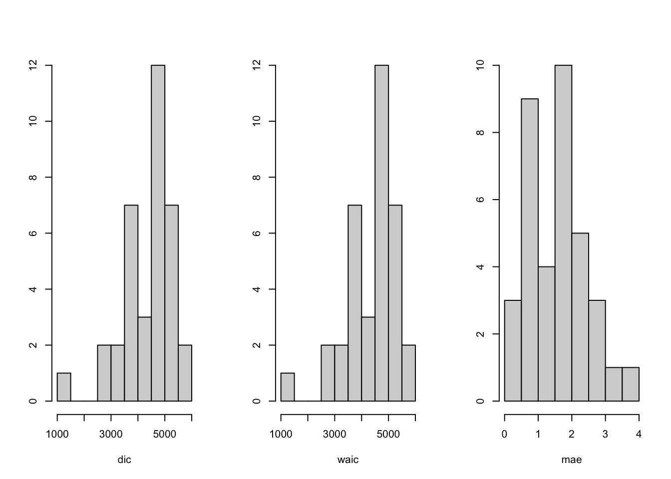
FIGURE 9.9: Histograms of model comparison criteria from Model Z1 across taxi zones.
Model Z2
Model Z2 is similar to Model Z1, except that the random intercept \(\beta_{t,0}\) is modeled as an AR(1) process instead of a random walk, i.e.,
\[\begin{align}
\beta_{t,0} &= \phi_0 \beta_{t-1,0}+ w_{t,0},
\tag{9.8}
\end{align}\]
where \(|\phi_0| <1\) and \(w_{t,0}\) is N\((0, \sigma^2_{w0})\). The code is similar to the code for Model Z1, except that we replace
f(id.t, model = "rw1", constr = FALSE) by f(id.t, model = "ar1") in the formula.
Details on the code and results are available on our GitHub link.
Model Z3
Model Z3 is obtained by dropping the deterministic trend term from Model Z1, so that
\[\begin{align} \log \lambda_{t} = \alpha + \beta_{t,0} + \sum_{j=1}^4 \beta_j Z_{t,j}. \tag{9.9} \end{align}\] The code is similar to the code for Model Z1, except that we replace the formula by
formula.zone.Z3 <- tnc ~ 1 +  costerm + sinterm + taxi + subway +
    f(id.t, model = "rw1", constr = FALSE)
The results from Model Z1–Z3 show that taxi zones ID127 and ID153 exhibit behavior that is very different than the other \(g_1 =34\) zones. We therefore exclude these zones when we fit the hierarchical model below.
Model Z4. Hierarchical model aggregating across zones
We fit a hierarchical version of Model Z1 with different levels \(\alpha_i\) to TNC usage data from \(g_1 = 34\) taxi zones, excluding zones ID127 and ID153.
\[\begin{align} y_{it}|\lambda_{it} &\sim \mbox{Poisson}(\lambda_{it}), \notag \\ \log \lambda_{it} &= \alpha_i + \gamma t + \beta_{it,0} + \sum_{j=1}^4 \beta_{j} Z_{it,j} \notag \\ \beta_{it,0} &= \beta_{i,t-1,0}+ w_{it,0}, \tag{9.10} \end{align}\] where \(w_{it,0} \sim N(0, \sigma^2_{w0})\).
ride.hzone <- ride.zone %>%
  filter(zoneid != "ID127" & zoneid != "ID153")
g1 <- n_distinct(ride.hzone$zoneid)
trend <- 1:n
htrend <- rep(trend, g1)
hcosterm <- rep(costerm, g1)
hsinterm <- rep(sinterm, g1)
Model Z4a
The levels \(\alpha_i\) are assumed to be fixed coefficients for the \(g_1 =34\) zones. Indexes, replicates, and the data frame for Model Z4a are set up below. The formula includes the levels as fixed effects using fact.alpha <- as.factor(id.alpha).
id.b0 <- rep(1:n, g1)
re.b0 <- id.alpha <- rep(1:g1, each = n)
fact.alpha <- as.factor(id.alpha)
ride.hzone.data.fe <-
  cbind.data.frame(ride.hzone, htrend, hcosterm, hsinterm, id.b0, re.b0,
                   fact.alpha)
formula.hzone.fe <-
  tnc ~ -1 + fact.alpha + htrend + hcosterm + hsinterm + taxi + subway +
  f(id.b0, model = "rw1", replicate = re.b0)
model.hzone.fe <- inla(
formula.hzone.fe,
data = ride.hzone.data.fe,
family = "poisson",
control.predictor = list(compute = TRUE, link = 1),
control.compute = list(dic = TRUE, waic = TRUE, cpo = TRUE)
)
#summary(model.hzone.fe)We show posterior summaries on a few of the estimated \(\alpha_i\) and other fixed effects and random hyperparameters.
summary.model.hzone.fe <- summary(model.hzone.fe)
format.inla.out(summary.model.hzone.fe$fixed[30:39,c(1,2)])
##    name         mean   sd
## 1  fact.alpha30  0.906 0.035
## 2  fact.alpha31  1.761 0.035
## 3  fact.alpha32  1.573 0.034
## 4  fact.alpha33  0.844 0.035
## 5  fact.alpha34  1.486 0.034
## 6  htrend        0.002 0.000
## 7  hcosterm     -0.021 0.002
## 8  hsinterm      0.062 0.002
## 9  taxi          0.009 0.000
## 10 subway        0.001 0.000
format.inla.out(summary.model.hzone.fe$hyperpar[,c(1,2)])
##   name                mean sd
## 1 Precision for id.b0 6767 420.5
To see the actual values of the posterior means and standard deviations of the coefficients of Taxi and Subway usage, we can use the code below:
tail(model.hzone.fe$summary.fixed[c(1,2)],2)## mean sd
## taxi 0.008904 8.055e-05
## subway 0.001205 6.041e-05Model Z4b
Since there are \(g_1=34\) zones, we may instead wish to treat the \(\alpha_i\) as random effects, i.e., \(\alpha_i \sim N(0,\sigma^2_\alpha)\), where \(\sigma^2_\alpha\) is unknown. The indexes, replicates, formula, and model fit are shown below.
id.b0 <- rep(1:n, g1)
re.b0 <- id.alpha <- rep(1:g1, each = n)
prec.prior <-
  list(prec = list(param = c(0.001, 0.001), initial = 20))
ride.hzone.data.re <-
  cbind.data.frame(ride.hzone, htrend, hcosterm, hsinterm, id.b0, re.b0,
                   id.alpha)
formula.hzone.re <-
  tnc ~ -1 + htrend + hcosterm + hsinterm + taxi + subway +
  f(id.alpha, model = "iid", hyper = prec.prior) +
  f(id.b0, model = "rw1", replicate = re.b0)
model.hzone.re <- inla(
formula.hzone.re,
family = "poisson",
data = ride.hzone.data.re,
control.predictor = list(compute = TRUE, link = 1),
control.compute = list(
dic = TRUE,
cpo = TRUE,
waic = TRUE,
config = TRUE,
cpo = TRUE
)
)
summary(model.hzone.re)summary.model.hzone.re <- summary(model.hzone.re)
format.inla.out(summary.model.hzone.re$fixed)
## name mean sd 0.025q 0.5q 0.975q mode kld
## 1 htrend 0.002 0.000 0.002 0.002 0.002 0.002 0
## 2 hcosterm -0.021 0.002 -0.025 -0.021 -0.017 -0.021 0
## 3 hsinterm 0.062 0.002 0.059 0.062 0.065 0.062 0
## 4 taxi 0.009 0.000 0.009 0.009 0.009 0.009 0
## 5 subway 0.001 0.000 0.001 0.001 0.001 0.001 0
format.inla.out(summary.model.hzone.re$hyperpar[,c(1,2)])
## name mean sd
## 1 Precision for id.alpha 0.575 0.142
## 2 Precision for id.b0 6752.865 425.638Boxplots of \(\alpha_i\)’s generated from inla.posterior.sample for Model Z4b are shown in Figure 9.10. The distribution of the level varies across zones.
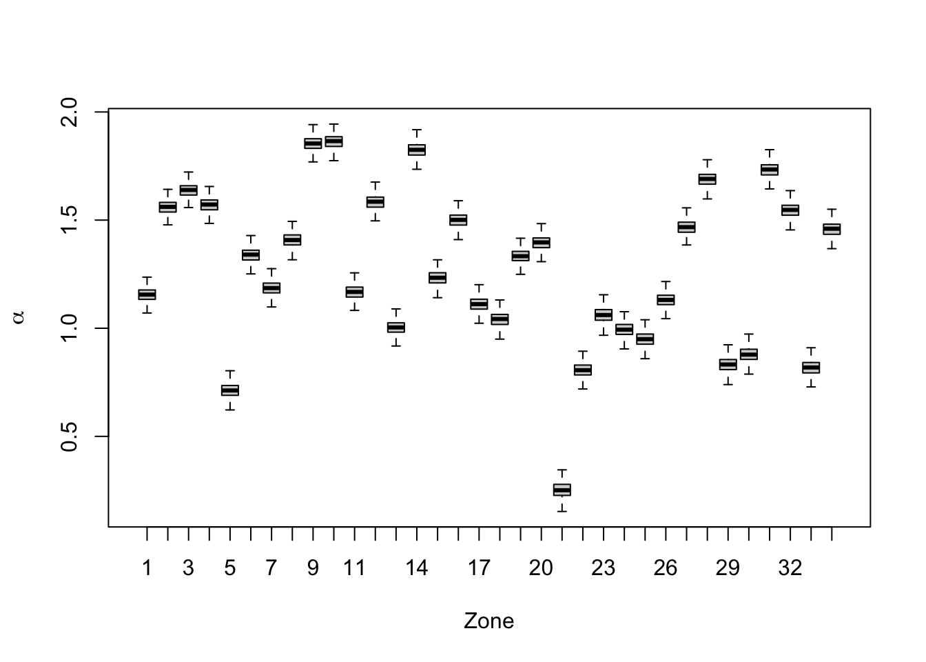
FIGURE 9.10: Boxplots of \(\alpha_i\)’s for 34 zones from Model Z4b.
In-sample comparison criteria for Models Z1 to Z4b are shown in Table 9.1.
| Model | DIC | WAIC | Average in-sample MAE |
|---|---|---|---|
| Model Z1 | 4418 | 4399 | 1.604 |
| Model Z2 | 4422 | 4403 | 1.616 |
| Model Z3 | 4427 | 4400 | 1.561 |
| Model Z4a | 159074 | 158597 | 2.168 |
| Model Z4b | 159074 | 158596 | 2.168 |
Remark. We can run similar hierarchical models corresponding to Model Z2 and Model Z3 (results not shown here) and compare the different models for TNC usage in the \(g_1 =34\) taxi zones.