Chapter 3 Details of R-INLA for Time Series

3.1 Introduction

In this chapter, we show how to use the R-INLA package for analyzing univariate time series. Specifically, we show how we set up the formula and model statements for analyzing a time series as a random walk, a random walk with drift, or autoregessions of various orders, excluding or including a level coefficient. R-INLA implements the integrated nested Laplace approximations that we discussed in Chapter 2 in order to carry out approximate Bayesian inference. We first show the details of Bayesian model fitting using R-INLA for time series simulated from a random walk plus noise model (also called the local level model), which was introduced in Chapter 1. We then discuss several other models for univariate time series. Further, we use these model fits to obtain future forecasts on hold-out (test) data. These forecasts can be used for predictive cross-validation and model selection. In practice, one can then use the best fitting model to forecast the time series into the future.

The first step is to install the package R-INLA:

install.packages(
  "INLA",
  repos = c(getOption("repos"),
            INLA = "https://inla.r-inla-download.org/R/stable"),
  dep = TRUE
)

Then, we source the package, along with other packages used in this chapter.

library(INLA)
library(tidyverse)

Next, the set of custom functions that we have built must be sourced so that they may be called at various places in the chapter.

source("functions_custom.R")

3.2 Random walk plus noise model

In Chapter 1, we defined the random walk plus noise model (also referred to as the local level model) using the observation equation and state equation shown in (1.15) and (1.16) as

\[\begin{align*} y_t &= x_t + v_t;~~ v_t \sim N(0, \sigma^2_v), \\ x_t &= x_{t-1}+ w_t;~~ w_t \sim N(0, \sigma^2_w), \end{align*}\] where \(x_0=0\), and \(v_t\) and \(w_t\) are uncorrelated errors, following zero mean normal distributions with unknown variances \(\sigma^2_v\) and \(\sigma^2_w\) respectively. The response variable is denoted by \(y_t\). The state variable \(x_t\) is a latent Gaussian variable. Let \(\boldsymbol{\theta}=(\sigma^2_v, \sigma^2_w)'\) denote the vector of unknown hyperparameters. This is a special case of the DLM shown in (1.17) and (1.18) with \(\alpha=0\), \(F_t =1\) and \(G_t=1\). We show the detailed steps for fitting this model to a simulated time series and verify that we are able to recover the true parameters that we used to generate the series. We set the length of the time series to be \(n=500\). The true parameter values for the observation error variance and state error variance are \(\sigma^2_v=0.5\) and \(\sigma^2_w=0.25\) respectively.

We simulate a time series from the model in (1.15) and (1.16) using the custom function simulation.from.rw1() which is included in the set of functions that we sourced in the introduction via

source("functions_custom.R")

To see a plot of the time series, use plot.data = TRUE. Figure 3.1 shows a wandering behavior which is typical of the nonstationary random walk series.

sim.rw1 <-
  simulation.from.rw1(
    sample.size = 500,
    burn.in = 100,
    level = 0,
    drift = 0,
    V = 0.5,
    W = 0.25,
    plot.data = TRUE,
    seed = 123457
  )
sim.rw1$sim.plot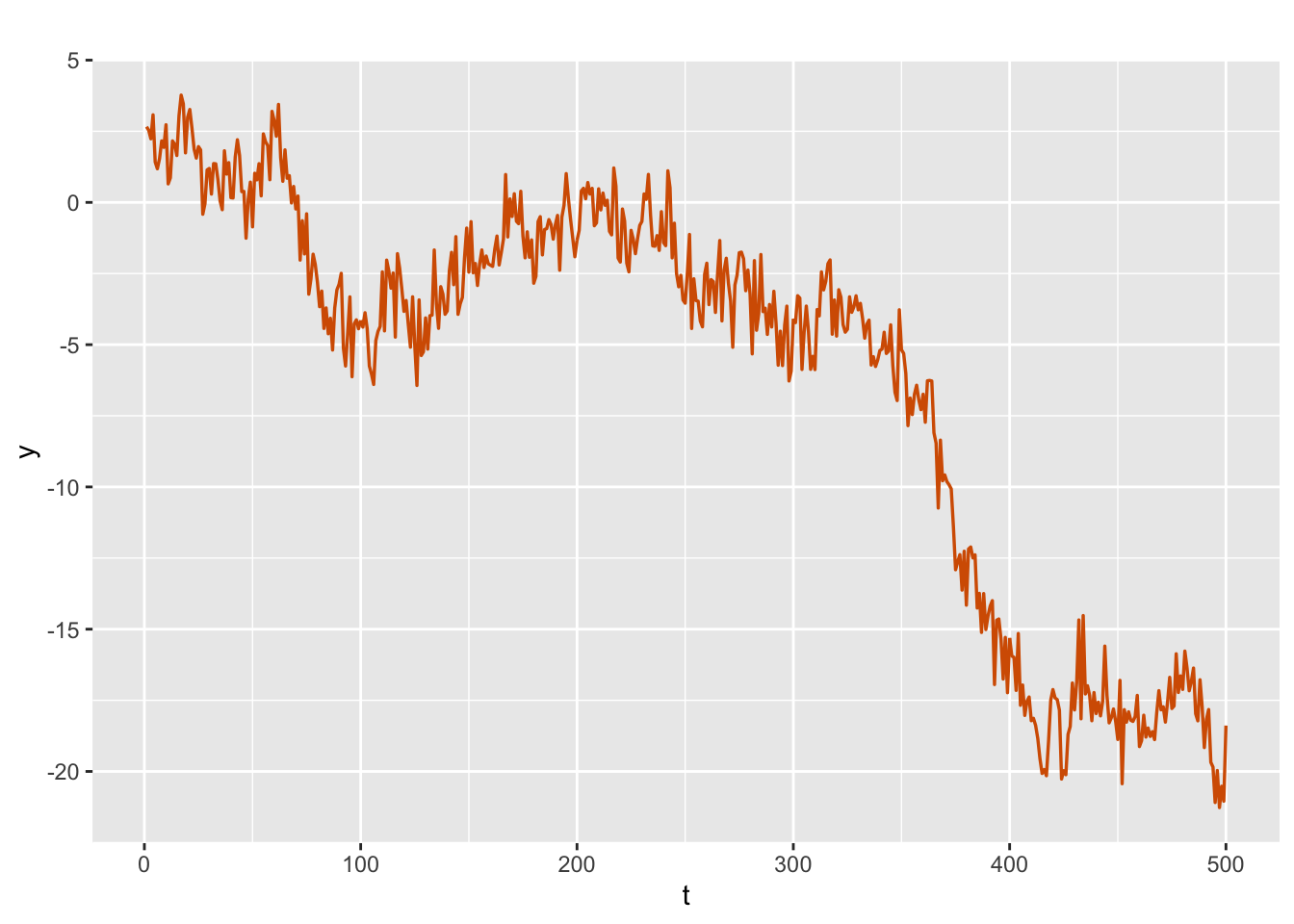

FIGURE 3.1: Simulated random walk plus noise series.

To use R-INLA for fitting this model to the data, we discuss three main components:

1. a formula to specify the model, similar to the formula in the R function lm() used to fit the usual linear regression model (see Section 3.2.1).

2. model execution, which is used to obtain results and posterior summaries (see Section 3.2.2), and

3. prior and hyperprior specifications, when relevant (see Section 3.2.3).

3.2.1 R-INLA model formula

The information in the observation and state equations of a DLM is represented as a formula, similar to the formula used in the R function lm(). We can specify time effects, and in general any structured effect, using a function f() within the formula. Examples of structured effects for univariate time series are iid, rw1, ar1, etc. The time effect is represented as an index in f(). Specifically, we set up a time index id.w that runs from \(1\) to \(n\), where \(n\) denotes the length of the time series. We then set up a data frame rw1.dat, with two columns containing the time series \(y_t\) and the time index id.w.

y.rw1 <- sim.rw1$sim.data
n <- length(y.rw1)
id.w <- 1:n
rw1.dat <- cbind.data.frame(y.rw1, id.w)

The model argument within the function f() is specified to be rw1. Since no intercept needs to be estimated in the observation equation (i.e., \(\alpha=0\)), we include “\(-1\)” in the formula; note that this usage is similar to the lm() function.

formula.rw1 <- y.rw1 ~ f(id.w, model = "rw1",
                         constr = FALSE) - 1

In the formula, constr is an option to let the sum of terms (in this case \(x_t\)) be zero, which is the default option in R-INLA. Using ?f(), we can get help on the constr option: “A boolean variable indicating whether to set a sum to 0 constraint on the term. By default the sum to 0 constraint is imposed on all intrinsic models (”iid”,”rw1”,”rw2”,”besag”, etc.).” We specify constr=FALSE, since there is no constraint in the random walk plus noise model. Information on all arguments available with the function f() can be accessed using ?f().

3.2.2 Model execution

We can fit the model using the function inla(). The general syntax is shown below, where formula was defined in the previous subsection.

inla(formula = ,family = ,data = ,control.compute = ,
  control.predictor = ,control.family = ,...)

For the Gaussian DLM, \(y_t\) has a normal distribution and we set family = gaussian.
In later chapters, we will look at examples of non-Gaussian families for \(y_t\), and specify these via the appropriate input in family =. Recall that the latent state variable \(x_t\) is always assumed to be Gaussian in this framework (see Chapter 2).

The data is set to be the data frame we created earlier, i.e., data = rw1.dat. R-INLA has several control options which enable a user to control different aspects of the modeling and output generation, and excellent documentation of these options is available on their website by using ?inla. For example, information on control.compute can be obtained from ?control.compute. Gómez-Rubio (2020) has presented a table with various options in control.compute; we show a similar display in Table 14.1. In the code below, we include the option control.predictor, which provides information on fitted values. In later sections of this chapter and in later chapters, we discuss other control options. In Chapter 14, we collect some of these items in a single place for quick reference.

model.rw1 <- inla(
  formula.rw1,
  family = "gaussian",
  data = rw1.dat,
  control.predictor = list(compute = TRUE)
)

The results from the inla() call shown above are stored in model.rw1, which is a list consisting of a number of objects. Before we do a deep dive into the output generated by inla(), we look at the detailed model summary, which is obtained using the function summary():

summary(model.rw1)
## 
## Call:
##    c("inla(formula = formula.rw1, family = \"gaussian\", data = 
##    rw1.dat, ", " control.predictor = list(compute = TRUE))") 
## Time used:
##     Pre = 4.29, Running = 0.825, Post = 0.425, Total = 5.54 
## Random effects:
##   Name     Model
##     id.w RW1 model
## 
## Model hyperparameters:
##                                         mean    sd 0.025quant
## Precision for the Gaussian observations 1.66 0.152       1.38
## Precision for id.w                      4.79 0.868       3.32
##                                         0.5quant 0.975quant mode
## Precision for the Gaussian observations     1.65       1.98 1.64
## Precision for id.w                          4.71       6.72 4.56
## 
## Expected number of effective parameters(stdev): 143.47(15.72)
## Number of equivalent replicates : 3.48 
## 
## Marginal log-Likelihood:  -750.25 
## Posterior marginals for the linear predictor and
##  the fitted values are computed

Description of the output

The output from summary() is very detailed, parts of which are self-explanatory, while others need some explanation. Below, we describe all the terms from the output.

1. call: the function called, with relevant arguments. Here,

summary(model.rw1)$call
## [1] "inla(formula = formula.rw1, family = \"gaussian\", data = rw1.dat, "
## [2] "    control.predictor = list(compute = TRUE))"

We can also obtain this using model.rw1$call.

2. Time used: time taken by the system to execute the model fit. Here,

summary(model.rw1)$cpu.used
## [1] "Pre = 4.29, Running = 0.825, Post = 0.425, Total = 5.54"

We can also obtain the same output by using model.rw1$cpu.used.

3. The model has no fixed effects: note that in the equations for the random walk plus noise model, \(x_t\) is time varying, and there are no “fixed” effects in the model (such as the intercept, \(\alpha\), say).

4. Random effects: in the model, \(x_t\) is a latent process and the structured effect rw1 is captured through the variable id.w. See

summary(model.rw1)$random.names
## [1] "id.w"
summary(model.rw1)$random.model
## [1] "RW1 model"

5. Model hyperparameters: a summary of parameter estimation corresponding to \(\sigma^2_v\) and \(\sigma^2_w\) is shown under this heading, and consists of the mean, standard deviation, \(2.5^{th}\) quantile, median, \(97.5^{th}\) quantile, and the mode of the posterior distributions of the following terms: precision for the Gaussian observations, i.e., the precision for \(v_t\), which is \(1/\sigma^2_v\), and precision for id.w, i.e., the precision of \(w_t\), which is \(1/\sigma^2_w\).

summary(model.rw1)$hyperpar
##                                          mean    sd 0.025quant
## Precision for the Gaussian observations 1.661 0.152      1.380
## Precision for id.w                      4.791 0.868      3.316
##                                         0.5quant 0.975quant  mode
## Precision for the Gaussian observations    1.654      1.978 1.643
## Precision for id.w                         4.712      6.720 4.559

We can also get this using model.rw1$summary.hyperpar; note the difference in the number of digits printed.

6. Expected number of effective parameters: this is the number of independently estimated parameters in the model.

summary(model.rw1)$neffp
##                                      [,1]
## Expectected  number of parameters 143.475
## Stdev of the number of parameters  15.719
## Number of equivalent replicates     3.485

7. Marginal log-likelihood: this was defined in Chapter 2 and is used in model selection, as discussed in Section 3.8.

summary(model.rw1)$mlik
##                                         [,1]
## log marginal-likelihood (integration) -750.0
## log marginal-likelihood (Gaussian)    -750.3

We can also obtain this using model.rw1$mlik.

8. Posterior marginals for linear predictor and fitted values: while calling the inla() function, we request this output through the option control.predictor = list(compute = TRUE).

head(summary(model.rw1)$linear.predictor)

This can also be obtained using model.rw1$summary.linear.predictor. It is useful to print a condensed summary for the fitted values:

head(summary(model.rw1)$linear.predictor)
##                mean    sd 0.025quant 0.5quant 0.975quant  mode kld
## Predictor.001 2.488 0.518      1.473    2.488      3.504 2.487   0
## Predictor.002 2.428 0.450      1.547    2.428      3.310 2.428   0
## Predictor.003 2.331 0.426      1.496    2.331      3.167 2.330   0
## Predictor.004 2.270 0.419      1.449    2.269      3.093 2.268   0
## Predictor.005 1.918 0.417      1.099    1.918      2.734 1.919   0
## Predictor.006 1.745 0.417      0.925    1.746      2.561 1.747   0

Condensed output

The output from inla() can be unwieldy. It is possible to show a condensed output by excluding selected columns from the detailed output, as we show below. Our function format.inla.out() requires the R package tidyverse (Wickham et al. 2019). For details on the tidyverse package and other data wrangling approaches, see Boehmke (2016). To show only the mean, standard deviation, and median of the hyperparameter distributions, we use

format.inla.out(model.rw1$summary.hyperpar[,c(1,2,4)])

##   name                       mean  sd    0.5q 
## 1 Precision for Gaussian obs 1.661 0.152 1.654
## 2 Precision for id.w         4.791 0.868 4.712

The condensed output below only shows the three quantiles from the hyperparameter distributions.

format.inla.out(model.rw1$summary.hyperpar[,c(3,4,5)])

  name                       0.025q 0.5q  0.975q
1 Precision for Gaussian obs 1.380  1.654 1.978 
2 Precision for id.w         3.316  4.712 6.720 

Below, we illustrate output only on the mean, median, and mode of the hyperparameter distributions.

format.inla.out(model.rw1$summary.hyperpar[,c(1,4,6)])

  name                       mean  0.5q  mode 
1 Precision for Gaussian obs 1.661 1.654 1.643
2 Precision for id.w         4.791 4.712 4.559

Although we only show condensed output in most places in the book due to space restrictions, a user may obtain and directly view the full output by excluding format.inla.out().

3.2.3 Prior specifications for hyperparameters

Setting prior specifications for the hyperparameters is an important step in the Bayesian framework. Data analysts often give considerable thought to specifying appropriate and reasonable priors. If a user does not wish to specify a custom prior distribution, R-INLA uses a default prior specification. In most situations, these default priors work quite well. Here, we talk about default priors available for hyperparameters (or model parameters) in a Gaussian DLM. In Section 3.9, we discuss how a user may set up non-default or custom priors (also see Chapter 5 in Gómez-Rubio (2020)).

It is important to note that R-INLA assigns priors via an internal representation for the parameters. This representation may not be the same as the scale of the parameter that is specified in the model by a user. For instance, precisions (which are reciprocals of variances) are represented on the log scale. In the Gausssian DLM, the precision corresponding to the observation noise variance is \(1/\sigma^2_v\), and R-INLA sets a prior for \(\theta_v = \log(1/\sigma^2_v)\). As explained in Rue, Martino, and Chopin (2009), the internal representation is computationally convenient, since the parameter is not bounded in the internal scale and has the entire real line \(\mathbb{R}\) as support. We next show how we set up and execute the model under default priors for observation and state noise variances via \(\theta_v = \log(1/\sigma^2_v)\) and \(\theta_w = \log(1/\sigma^2_w)\).

Default priors for \(\sigma^2_v\) and \(\sigma^2_w\)

To define the prior specification corresponding to the observation noise variance \(\sigma^2_v\), consider the corresponding log precision

\[\begin{align*} \theta_v = \log\left(\frac{1}{\sigma^2_v}\right), \end{align*}\] and let

\[\begin{align*} \theta_v \sim {\rm log~gamma}({\rm shape} =1, {\rm inverse~scale = 5e-05}). \end{align*}\]
The logarithm of the precision \(\theta_v\) is assumed by default to follow a log-gamma distribution. The shape and inverse scale parameters of this log-gamma prior are unknown, and by default, R-INLA assigns to them the values \(1\) and 5e-05 respectively. The default initial value for this log-gamma hyperparameter is set as \(4\).

Similarly, a default log-gamma prior with values \(1\) and 5e-05 for the shape and inverse scale and a default initial value of \(4\) is specified for \(\theta_w = \log(1/\sigma^2_w)\), the logarithm of the reciprocal of the state error variance \(\sigma^2_w\). That is, we let

\[\begin{align*} \theta_w = \log\left(\frac{1}{\sigma^2_w}\right), \end{align*}\] and
\[\begin{align*} \theta_w \sim {\rm log~gamma}({\rm shape} =1, {\rm inverse~scale = 5e-05}). \end{align*}\] More details on these default prior specifications for this model can be accessed from the INLA documentation inla.doc("rw1").

3.2.4 Posterior distributions of hyperparameters

We can obtain marginal posterior distributions of the latent variables (treated as parameters) \(x_t\) and the hyperparameters \(\boldsymbol{\theta}\), and manipulate these distributions. The options are summarized in Table 14.2, which shows the different functions and their descriptions (similar to the one displayed in Gómez-Rubio (2020)).

We have seen that R-INLA works with the log precisions of hyperparameters rather than their variances. Therefore, in order to obtain marginal posterior distributions of \(\sigma^2_v\) and \(\sigma^2_w\), we must transform each log(precision) back to the corresponding variance using the function inla.tmarginal(). The result for \(\sigma^2_v\) is shown in Figure 3.2.

sigma2.v.dist <- inla.tmarginal(
  fun = function(x)
    exp(-x),
  marginal = model.rw1$
  internal.marginals.hyperpar$`Log precision for the Gaussian observations`
)
plot(
  sigma2.v.dist,
  type = "l",
  xlab = expression(paste(
    "Observation noise variance ", sigma[v] ^ 2, sep = " "
  )),
  ylab = "density"
)

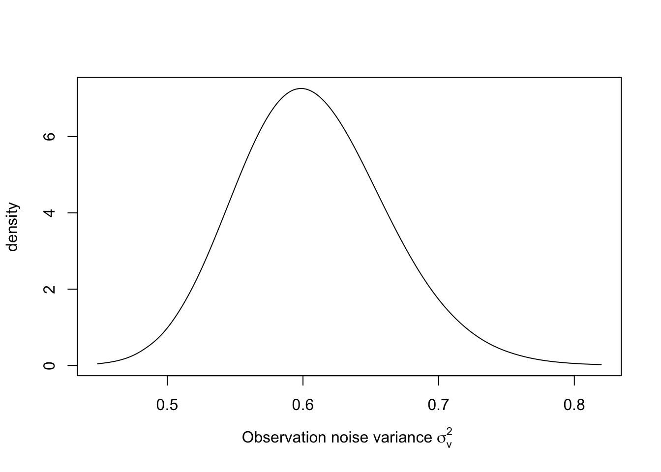
FIGURE 3.2: Posterior distribution of \(\sigma^2_v\) in the random walk plus noise model.

The marginal posterior for \(\sigma^2_w\) may be similarly obtained, see Figure 3.3.

sigma2.w.dist <- inla.tmarginal(
  fun = function(x)
    exp(-x),
  marginal = model.rw1$internal.marginals.hyperpar$`Log precision for id`
)
plot(sigma2.w.dist,
     type = "l",
      xlab = expression(paste(
    "State noise variance ", sigma[w]^2, sep = " "
  )),
     ylab = "density")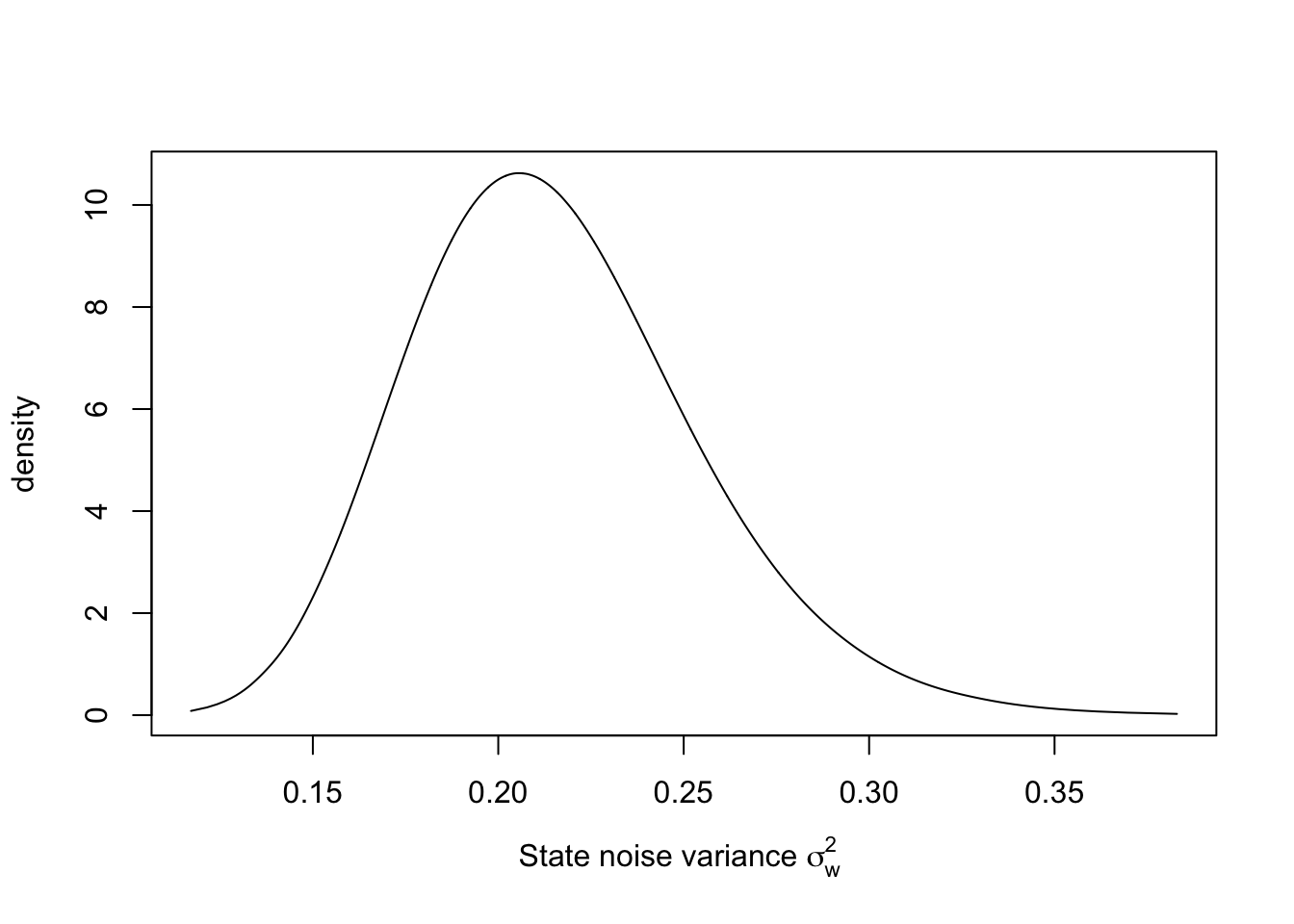

FIGURE 3.3: Posterior distribution of \(\sigma^2_w\) in the random walk plus noise model.

R-INLA incorporates several functions to manipulate the posterior marginals. For example, inla.emarginal() and inla.qmarginal() respectively calculate the expectation and quantiles of the marginal posteriors. The function inla.smarginal() can be used to do spline smoothing, inla.tmarginal() can be used to transform the marginals, and inla.zmarginal() provides summary statistics.

We can write the posterior expectations of \(\sigma^2_v\) and \(\sigma^2_w\).

sigma2.v.hat <-
  inla.emarginal(
    fun = function(x)
      exp(-x),
    marginal = model.rw1$internal.marginals.hyperpar$
      `Log precision for the Gaussian observations`
  )
sigma2.w.hat <-
  inla.emarginal(
    fun = function(x)
      exp(-x),
    marginal = model.rw1$internal.marginals.hyperpar$`Log precision for id`
  )
cat(paste(
  "Estimated observation noise variance, sigma2.v",
  round(sigma2.v.hat, 2),
  sep = " = "
),
"\n")
## Estimated observation noise variance, sigma2.v = 0.61
cat(paste(
  "Estimated state noise variance, sigma2.w",
  round(sigma2.w.hat, 2),
  sep = " = "
))
## Estimated state noise variance, sigma2.w = 0.22

3.2.5 Fitted values for latent states and responses

We describe how we recover the fitted state variables \(x_t\) and the fitted responses \(y_t\) for each time \(t=1,\ldots,n\). The fitted state variable from R-INLA corresponds to the smoothed estimate of \(x_t\), as we discuss below.

Fitted values for the state variables \(x_t\)

For \(t=1,\ldots,n\), fitted values of the state variable \(x_t\) are obtained as the means of the posterior distributions of \(x_t\) given all the data \({\boldsymbol y}^n=(y_1,\ldots, y_n)'\), i.e., \(\pi(x_t \vert {\boldsymbol y}^n)\). Posterior summaries of the state variable (the local level variable in the case of the random walk plus noise model) \(x_t\) are stored in summary.random. We display the first few rows below.

head(model.rw1$summary.random$id.w)
##   ID  mean     sd 0.025quant 0.5quant 0.975quant  mode       kld
## 1  1 2.488 0.5178     1.4718    2.488      3.505 2.487 8.692e-08
## 2  2 2.428 0.4497     1.5453    2.428      3.311 2.428 1.188e-07
## 3  3 2.331 0.4262     1.4943    2.331      3.168 2.330 9.244e-08
## 4  4 2.270 0.4191     1.4475    2.269      3.093 2.268 1.318e-07
## 5  5 1.918 0.4166     1.0983    1.918      2.734 1.919 8.678e-08
## 6  6 1.745 0.4170     0.9234    1.746      2.561 1.747 2.460e-07

A condensed output is shown below.

format.inla.out(head(model.rw1$summary.random$id[,c(1:5)]))
##   ID mean  sd    0.025q 0.5q 
## 1 1  2.488 0.518 1.472  2.488
## 2 2  2.428 0.450 1.545  2.428
## 3 3  2.331 0.426 1.494  2.331
## 4 4  2.270 0.419 1.448  2.269
## 5 5  1.918 0.417 1.098  1.918
## 6 6  1.745 0.417 0.923  1.746

In the usual Gaussian DLM terminology, these estimates are called the Kalman smoothed estimates or simply, the smooth (Shumway and Stoffer 2017), and are obtained for \(t=1,\ldots,n\) using just one inla() call. By default, R-INLA uses a simplified Laplace approximation (see Chapter 2 for a description). For each \(t\), posterior summaries of \(\pi(x_t \vert {\boldsymbol y}^n)\) are given, along with the Kullback-Leibler Divergence (KLD) defined in (2.17). The KLD gives the distance between the standard Gaussian distribution and the simplified Laplace approximation to the marginal posterior densities (see Chapter 2 – Appendix for a description).

A plot of the posterior means of \(x_t\) over time together with the 2.5th and 97.5th percentiles for the random walk plus noise model is shown in Figure 3.4.

plot.data <- model.rw1$summary.random$id %>%
  select(time = ID, mean,
         "0.025quant", "0.975quant")
multiline.plot(plot.data, xlab = "t", ylab = "posterior mean",
               line.color = c("black", "red", "red"),
               line.size = 0.6)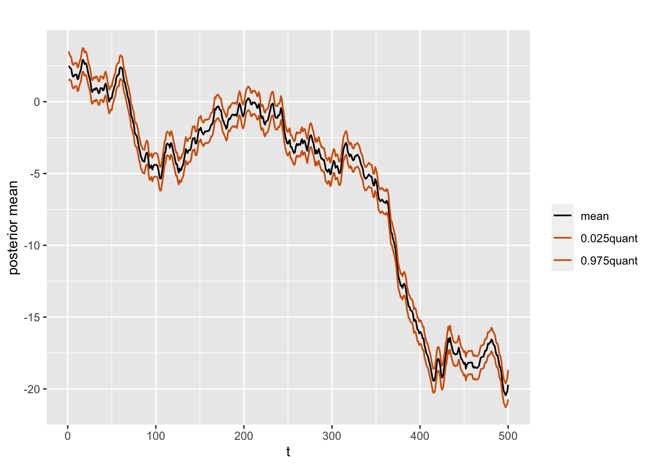

FIGURE 3.4: Posterior means and percentiles of the state variable over time in the random walk plus noise model.

For plotting multiple lines, we have used a customized function called multiline.plot(), which uses the R package ggplot2 (Wickham 2016). A summary of this function and other customized functions is shown in Chapter 14.

Fitted values for \(y_t\)

For \(t=1,\ldots,n\), the fitted values of \(y_t\) are the posterior means of the predictive distributions of \(y_t\) given \({\boldsymbol y}^n = (y_1,\ldots, y_n)'\) and can be retrieved by using the code below; see Figure 3.5 for a plot. As we discussed in Chapter 2, for Gaussian response models (where the link is the identity link), we can use either the summary.linear.predictor or the summary.fitted.values in the control.predictor option in inla(), setting compute = TRUE.

fit <- model.rw1$summary.linear.predictor$mean
df <- as_tibble(cbind.data.frame(time = 1:n, y.rw1, fit))
multiline.plot(
  plot.data = df,
  title = "",
  xlab = "t",
  ylab = "y",
  line.type = "dashed",
  line.color = c("red", "blue"),
  line.size = 0.6
)

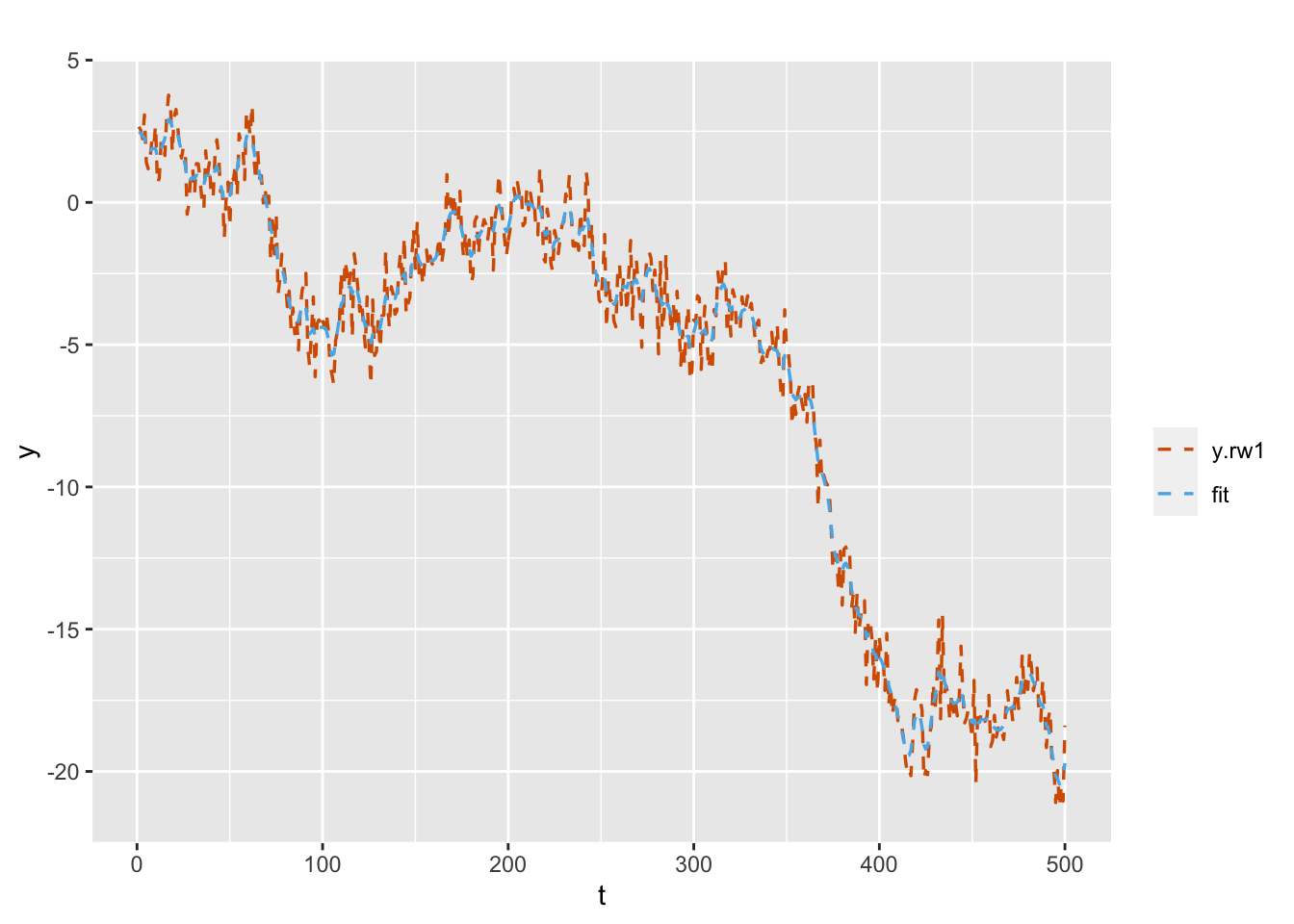
FIGURE 3.5: Simulated and fitted responses under the random walk plus noise model.

Two other approaches to obtain the fitted values are shown below. For Gaussian DLMs, each of these three ways gives exactly the same results. Other summaries such as standard deviation (sd) or quantiles can be obtained similarly. However, for non-Gaussian DLMs, note that we cannot use summary.linear.predictor, but can instead use one of the two alternate approaches shown below. We will revisit this in Chapter 9 for count time series. See ?inla for more details.

fit.alt.1 <- model.rw1$summary.fitted.values$mean
fit.alt.2 <- model.rw1$marginals.linear.predictor %>% 
  sapply(function(x) inla.emarginal(fun = function(y) y, marginal =x))

3.2.6 Filtering and smoothing in DLM

As we mentioned in Chapter 1, the Kalman filtering algorithm is a recursive algorithm to estimate the state variable \(\boldsymbol{x}_t\) in a DLM given data/information up to time \(t\), i.e., given \({\boldsymbol y}^t\) (Shumway and Stoffer 2017). Using this algorithm, a time series analyst is able to compute filter estimates of \(\boldsymbol{x}_t\) for \(t=1,\ldots,n\). Kalman filtering thus enables recursive estimation of the state variable as information comes in sequentially over time. It is well known that Kalman smoothing, on the other hand, estimates \(\boldsymbol{x}_t\) for times \(t = 1,\ldots,n\) given all the data \({\boldsymbol y}^n\). When we use R-INLA to fit a DLM, it returns the smoothed estimates of \(\boldsymbol{x}_t,~t=1,\ldots,n\). The posteriors of interest are therefore also approximated using all the information \({\boldsymbol y}^n\). The forward recursion to obtain filter estimates and backward recursions to obtain the smoothed estimates underlies Kalman’s algorithm (Kalman (1960)). These estimates are then used to recursively estimate the states and the hyperparameters. As discussed in Ruiz-Cárdenas, Krainski, and Rue (2012), a recursive (or sequential) approach for estimation and prediction is necessary in online (or real-time) settings as each new observation arrives, for instance in computer vision, finance, IoT monitoring systems, real-time traffic monitoring, etc. In these examples, it is useful to obtain filter estimates of the state variable \(x_t\), and then obtain the corresponding fits for \(y_t\).

The INLA approach argues that the estimation need not be recursive (or dynamic) in situations where all \(n\) observations in the time series are available rather than trickling in sequentially. The posteriors of interest are directly approximated in a non-sequential manner. While filter estimates of the state variable cannot be directly output in R-INLA, we can obtain filter estimates for \(x_t,~t=1,\ldots,n\) by repeatedly calling the inla() function \(n\) times. This is clearly a computationally expensive exercise, and when possible, it is useful to run the \(n\) inla() calls in parallel. We implement the parallel runs using the R package doParallel().

We obtain filter estimates of \(x_t\) from the random walk plus noise model, using the series \(y_t\) that we simulated earlier in this section; see Figure \(\ref{fig:rw1filter}\). The custom function to obtain the filter estimates, filt.inla(), is shown in Section 14.3 and is included in the set of functions we sourced at the beginning of the chapter. Compared with the smoothed estimates for \(x_t\), computation of the filter estimates is time-consuming as expected (since we call inla() \(n\) times).

out <-
  filt.inla(
    data.series = y.rw1,
    model = "rw1",
    trend = "no",
    alpha = "no"
  )

filt.all.rw1 <- out$filt.all.bind 
filt.estimate.rw1 <- c(NA, filt.all.rw1$mean)
smooth.est <- model.rw1$summary.random$id$mean
plot.df <- as_tibble(cbind.data.frame(time = id.w,
                                      y = y.rw1,
                                      filter = filt.estimate.rw1,
                                      smooth = smooth.est))
multiline.plot(plot.df,
               title = "",
               xlab = "t",
               ylab = " ", line.type = "solid", line.size = 0.6, 
               line.color = c("red", "yellow", "green"))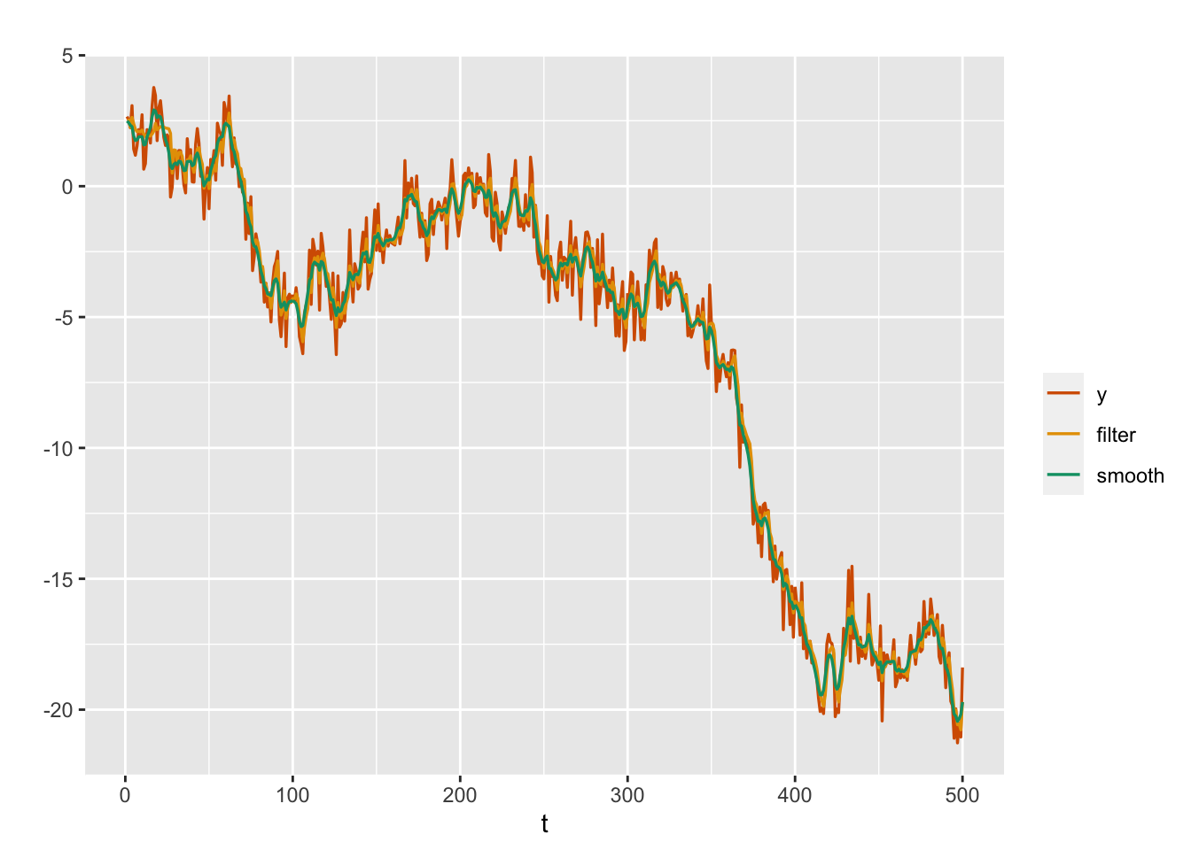

FIGURE 3.6: Simulated responses (red), with filtered (yellow) and smoothed (green) estimates of the state variable in the random walk plus noise model.

3.3 AR(1) with level plus noise model

In Chapter 1, we defined the AR(1) plus noise model using the observation and state equations (1.19) and (1.20). Here, we describe the R-INLA fit for an AR(1) with level plus noise model defined by the following DLM equations:

\[\begin{align} y_t &= \alpha + x_t + v_t;~~ v_t \sim N(0, \sigma^2_v), \tag{3.1}\\ x_t &= \phi x_{t-1} + w_t;~~ w_t \sim N(0, \sigma^2_w), ~ t=2,\ldots,n, \tag{3.2} \end{align}\] and

\[\begin{align} x_1 \sim N(0, \sigma^2_w/(1-\phi^2)), \tag{3.3} \end{align}\] where \(\vert \phi \vert <1\) and \(\alpha\) is the level parameter. Let \(\tau = 1/\sigma^2_w\) and \(\kappa = \tau (1-\phi^2) = (1-\phi^2)/\sigma^2_w\) denote the marginal precision of the state \(x_t\).

Note: R-INLA uses the notation \(\rho\) instead of \(\phi\) in the AR(1) model. In the output, when we see Rho, it refers to \(\phi\) in our notation.

We use the custom function simulation.from.ar() to simulate \(n=500\) values \(x_t\) from a Gaussian AR(1) process with \(\sigma^2_w=0.1\) and \(\phi=0.6\). This is done using the R function arima.sim(). We add \(\alpha=1.4\) and Gaussian errors \(v_t\) with variance \(\sigma^2_v=0.2\) to \(x_t\) in order to get the process \(y_t\); see Figure @ref{fig:ar1levelnoise}.

sim.ar1.level <-
  simulation.from.ar(
    sample.size = 500,
    burn.in = 100,
    phi = 0.6,
    level = 1.4,
    drift = 0,
    V = 0.2,
    W = 0.1,
    plot.data = TRUE,
    seed = 123457
  )
sim.ar1.level$sim.plot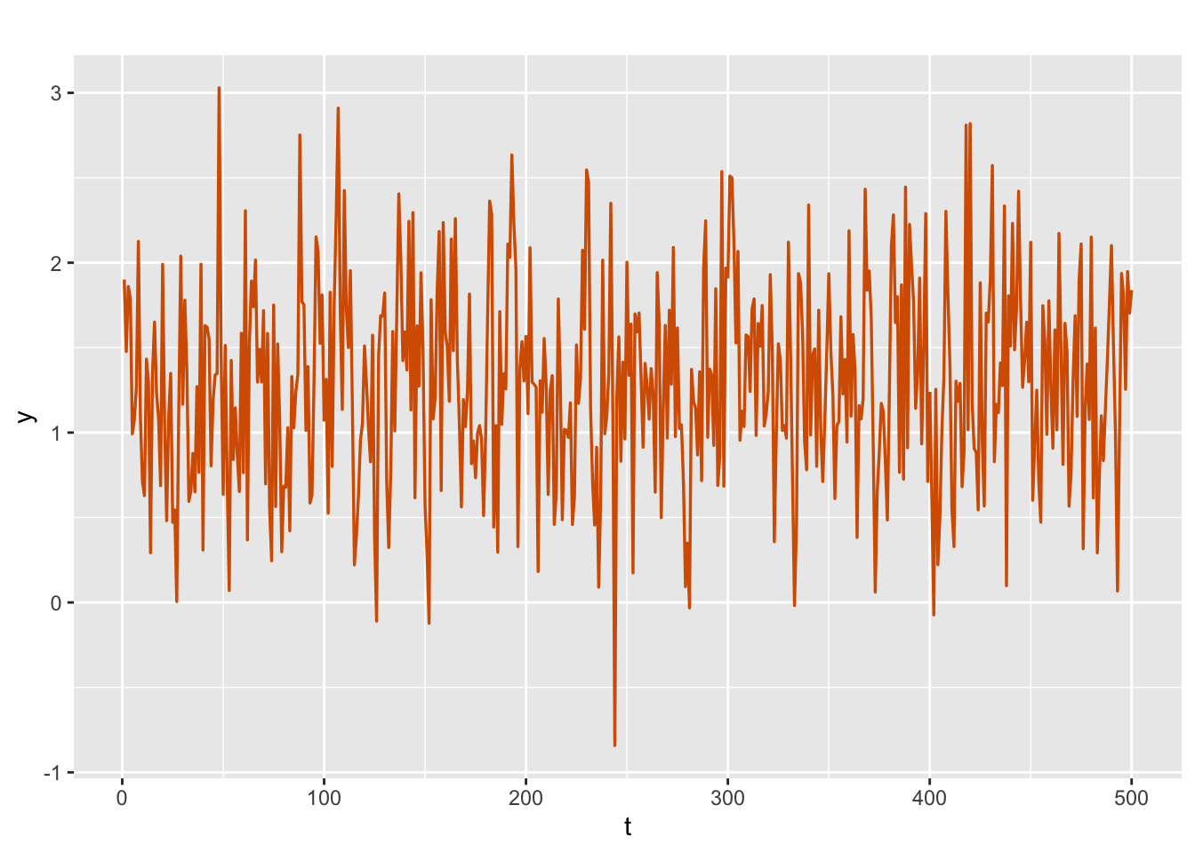

FIGURE 3.7: Simulated AR(1) with level plus noise series.

We next describe hyperparameter prior specifications. Let

\[\begin{align} \theta_v & = \log(1/\sigma^2_v), \quad \theta_w = \log \kappa = \log \left( \frac{1-\phi^2}{\sigma^2_w}\right), \notag \\ \theta_\phi & = \log \frac{1+\phi}{1-\phi}, \tag{3.4} \end{align}\] and let \(\boldsymbol\theta = (\theta_v,\theta_w,\theta_\phi)'\) be the internal representation of the hyperparameters. The default priors on \(\theta_v\) and \(\theta_w\) are log-gamma priors with shape and inverse scale being \(1\) and 5e-05, and default initial values of \(4\) in each case. Assume that

\[\begin{align*} \theta_\phi \sim N({\rm mean} =0, {\rm precision}=0.15); \end{align*}\] the normal prior depends on the mean and precision (reciprocal of the variance) parameters. R-INLA sets default values of \(0\) and \(0.15\) respectively for these values, while the initial value of \(\theta_\phi\) is assumed to be \(2\). For more details on the default prior specifications, see the R-INLA documentation inla.doc("ar1") and Chapter 5 of Gómez-Rubio (2020). The prior for the level parameter (intercept) \(\alpha\) is assumed to be a normal distribution with mean \(0\) and precision \(0.001\). For more details on this, see the R-INLA documentation for ?control.fixed. The code for model fitting is similar to the rw1 example, except that we now give a formula for an AR(1) model by inserting formula.ar1.level as the first item in the call to inla():

y.ar1.level <- sim.ar1.level$sim.data
n <- length(y.ar1.level)
id.x <- 1:n
data.ar1.level <- cbind.data.frame(y.ar1.level, id.x)
formula.ar1.level <-
  y.ar1.level ~ f(id.x, model = "ar1", constr = FALSE)
model.ar1.level <- inla(
  formula.ar1.level,
  family = "gaussian",
  data = data.ar1.level,
  control.predictor = list(compute = TRUE)
)
# summary(model.ar1.level)
format.inla.out(model.ar1.level$summary.hyperpar[,c(1:2)])
##   name                       mean  sd   
## 1 Precision for Gaussian obs 4.509 0.591
## 2 Precision for id.x         8.170 1.853
## 3 Rho for id.x               0.450 0.075
format.inla.out(model.ar1.level$summary.hyperpar[,c(3:5)])
##   name                       0.025q 0.5q  0.975q
## 1 Precision for Gaussian obs 3.389  4.496  5.748
## 2 Precision for id.x         5.277  7.898 12.634
## 3 Rho for id.x               0.301  0.450  0.597

We can then explore the posterior estimates of \(\sigma^2_v\), \(Var(x_t)=\sigma^2_x\), \(\phi\), and \(\alpha\), using code similar to that in the rw1 example. Specifically, for the AR(1) coefficient \(\phi\), the inverse transformation from \(\theta_\phi\) to \(\phi\) is obtained as

\[\begin{align} \phi = \frac{2 \exp(\theta_\phi)}{1+\exp(\theta_\phi)} -1. \tag{3.5} \end{align}\]

For an AR(1) model, note that R-INLA returns the precision of \(x_t\) i.e., \(1/{\rm Var}(x_t)\). This is different from the output we saw earlier for the rw1 model, where inla() returns the precision of the state error, \(1/\sigma^2_w\). For the variance of the state variable, \({\rm Var}(x_t)\), we have

var.x.dist <-  inla.tmarginal(
  fun = function(x)
    exp(-x),
  marginal = 
    model.ar1.level$internal.marginals.hyperpar$`Log precision for id`
)
var.x.zm <- inla.zmarginal(var.x.dist)
## Mean            0.128389 
## Stdev           0.027596 
## Quantile  0.025 0.0799905 
## Quantile  0.25  0.10859 
## Quantile  0.5   0.126634 
## Quantile  0.75  0.145925 
## Quantile  0.975 0.187606

The level (or intercept) is a fixed effect in this model. We can recover a summary of the fixed effect using

format.inla.out(model.ar1.level$summary.fixed[,c(1:5)])
##   name      mean  sd    0.025q 0.5q  0.975q
## 1 Intercept 1.287 0.034 1.221  1.287 1.354

The Highest Posterior Density (HPD) interval (D. Gamerman and Lopes 2006) for \(\alpha\) is

inla.hpdmarginal(0.95, model.ar1.level$marginals.fixed$`(Intercept)`)
##              low  high
## level:0.95 1.221 1.353

An alternate way to obtain posterior summaries for the fixed effect is given below.

alpha.fe <-  inla.tmarginal(
  fun = function(x)
    x,
  marginal = model.ar1.level$marginals.fixed$`(Intercept)`
)
alpha.fe.zm <- inla.zmarginal(alpha.fe, silent = TRUE)
alpha.hpd.interval <- inla.hpdmarginal(p = 0.95, alpha.fe)

The fitted values for \(x_t\) and \(y_t\) for the AR(1) with level plus noise model can be obtained using a code similar to that for the rw1 model. This is available on the GitHub link associated with the book.

It is useful to illustrate the effect of ignoring the level \(\alpha\) in fitting the model. While the correct (simulated) model is (3.1) and (3.2), suppose instead that a user fits a model without level by using the formula shown below.

formula.ar1.nolevel <-
  y.ar1.level ~ -1 + f(id.x, model = "ar1", constr = FALSE)
model.ar1.nolevel <- inla(
  formula.ar1.nolevel,
  family = "gaussian",
  data = data.ar1.level,
  control.predictor = list(compute = TRUE)
)
# summary(model.ar1.nolevel)
format.inla.out(model.ar1.nolevel$summary.hyperpar[,c(1:2)])
##   name                       mean  sd   
## 1 Precision for Gaussian obs 2.843 0.181
## 2 Precision for id.x         3.100 1.791
## 3 Rho for id.x               1.000 0.000
format.inla.out(model.ar1.nolevel$summary.hyperpar[,c(3:5)])
##   name                       0.025q 0.5q  0.975q
## 1 Precision for Gaussian obs 2.504  2.837 3.217 
## 2 Precision for id.x         0.844  2.715 7.642 
## 3 Rho for id.x               0.998  1.000 1.000

Note that as a consequence of omitting \(\alpha\) in the modeling, the estimate of the coefficient \(\phi\) tends to \(1\), which would indicate a latent random walk dependence! To avoid this, we recommend that a user always fits a model which includes a level \(\alpha\) in the observation equation. Of course, this coefficient will be estimated close to \(0\) when the level in the time series is zero.

3.4 Dynamic linear models with higher order AR lags

In R-INLA, we can assume that the latent Gaussian process \(x_t\) is an autoregressive process of order \(p\) (i.e., an AR\((p)\) process) for \(p \ge 1\), as described below.

AR\((p)\) with level plus noise model

Assume that the latent process \(x_t\) follows a stationary Gaussian AR\((p)\) process

\[\begin{align} \phi(B) x_t = (1-\phi_1 B - \phi_2 B^2 -\ldots - \phi_p B^p) x_t = w_t, \tag{3.6} \end{align}\] where \(w_t \sim N(0,\sigma^2_w)\), and the AR coefficients \(\phi_1, \phi_2,\ldots, \phi_p\) satisfy the stationarity condition, i.e., the modulus of each root of the AR polynomial equation \(\phi(B)= 0\) is greater than 1. See Chapter 3 – Appendix for more details, such as a definition of the backshift operator \(B\), and checking the stationarity conditions using the polyroot() function in R.

The AR\((p)\) with level plus noise model for \(y_t\) is defined as follows:

\[\begin{align} y_t &= \alpha + x_t + v_t;~~ v_t \sim N(0, \sigma^2_v), \tag{3.7} \\ x_t &= \sum_{j=1}^p \phi_j x_{t-j} + w_t;~~ w_t \sim N(0, \sigma^2_w), \tag{3.8} \end{align}\] where, \(\alpha\) is the level; we assume that \(x_0= x_{-1}=\ldots=x_{1-p}=0\), and the errors \(v_t\) and \(w_t\) follow zero mean normal distributions with unknown variances \(\sigma^2_v\) and \(\sigma^2_w\) respectively. R-INLA parameterizes the AR\((p)\) process in terms of the partial autocorrelations (see Chapter 3 – Appendix). When \(p=2\),

\[\begin{align} r_1 = \phi_1/(1 - \phi_2), \mbox{ and } ~r_2 = \phi_2, \tag{3.9} \end{align}\] R-INLA estimates these together with the error precisions \(1/\sigma^2_v\) and \(1/\sigma^2_w\). Using the inverse of this 1-1 transformation (see (3.40) in Chapter 3 - Appendix), we can recover the estimates of \(\boldsymbol{\phi} = (\phi_1,\ldots,\phi_p)'\). These steps are shown below for an AR\((2)\) model.

Example: AR(2) with level plus noise model

We simulate an AR(2) with level plus noise model with true values \(\phi_1=1.5\) and \(\phi_2=-0.75\) (corresponding to a stationary process), level \(\alpha=10\), and error variances \(\sigma^2_v=1.25\) and \(\sigma^2_w=0.05\). The plot of simulated series is shown in Figure 3.8.

sim.ar2 <-
  simulation.from.ar(
    sample.size = 500,
    burn.in = 100,
    phi = c(1.5,-0.75),
    level = 10,
    drift = 0,
    V = 1.25,
    W = 0.05,
    plot.data = TRUE,
    seed = 123457
  )
sim.ar2$sim.plot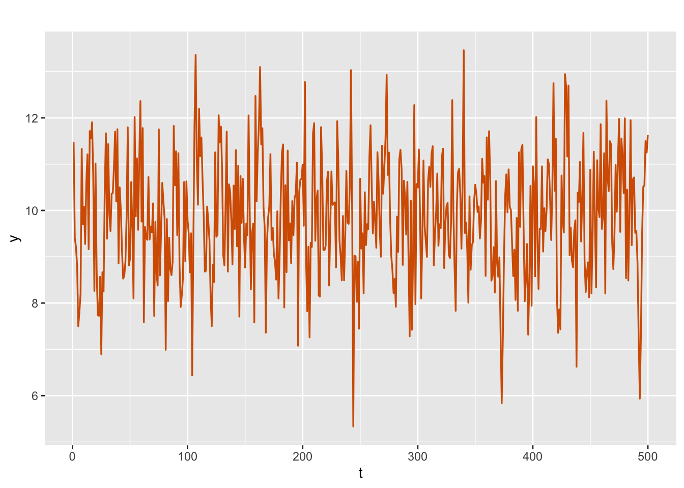

FIGURE 3.8: Simulated AR(2) with level plus noise series.

The 1-1 transformation in (3.9) can be written as

\[\begin{align*} \phi_1 = r_1 (1-r_2), \mbox{ and } \phi_2 = r_2. \end{align*}\] The model fitting is shown below.

y.ar2 <- sim.ar2$sim.data
n <- length(y.ar2)
id.x <- 1:n
ar2.dat <- cbind.data.frame(y.ar2, id.x)
formula.ar2 <- y.ar2 ~  f(id.x,
                     model = "ar",
                     order = 2,
                     constr = FALSE) 
model.ar2 <- inla(
  formula.ar2,
  family = "gaussian",
  data = ar2.dat,
  control.predictor = list(compute = TRUE)
)
# summary(model.ar2)
format.inla.out(model.ar2$summary.hyperpar[,c(1:2)])
##   name                       mean   sd   
## 1 Precision for Gaussian obs  0.808 0.062
## 2 Precision for id.x          2.106 0.481
## 3 PACF1 for id.x              0.856 0.021
## 4 PACF2 for id.x             -0.743 0.074
format.inla.out(model.ar2$summary.hyperpar[,c(3:5)])
##   name                       0.025q 0.5q   0.975q
## 1 Precision for Gaussian obs  0.692  0.806  0.937
## 2 Precision for id.x          1.335  2.047  3.215
## 3 PACF1 for id.x              0.812  0.857  0.893
## 4 PACF2 for id.x             -0.863 -0.752 -0.572

We can recover the summary of the fixed level \(\alpha\) using

format.inla.out(model.ar2$summary.fixed[,c(1:5)])
##   name      mean  sd    0.025q 0.5q  0.975q
## 1 Intercept 9.843 0.067 9.712  9.843 9.974

The inverse of the 1-1 transformation (3.40) enables us to recover the estimated \(\phi_1\) and \(\phi_2\) coefficients from the estimated partial autocorrelations, using the following functions:

pacf <- model.ar2$summary.hyperpar$mean[3:4]
phi <- inla.ar.pacf2phi(pacf)
print(phi)
## [1]  1.491 -0.743

We see that these values \(\hat{\phi}_1 =\) 1.491 and \(\hat{\phi}_2 =\) \(-0.743\) are close to the true values \(\phi_1=1.5\) and \(\phi_2= -0.75\). We can recover the variance of the state error \(w_t\) as follows. Recall that the Wold representation (or the MA\((\infty)\) representation) of a stationary AR\((p)\) process (3.6) is given by (see Shumway and Stoffer (2017))

\[\begin{align} x_t = \phi^{-1}(B) w_t = \sum_{j=0}^\infty \psi_j w_{t-j}, \tag{3.10} \end{align}\] where the weights in the infinite order polynomial \(\psi(B) = \sum_{j=0}^\infty \psi_j B^j\) are obtained by solving \(\psi(B) \phi(B)=1\). Then,

\[\begin{align} {\rm Var}(x_t) = \sigma^2_w \sum_{j=0}^\infty \psi_j^2. \tag{3.11} \end{align}\] We use the R function ARMAtoMA() to get a large number (here, \(100\)) of \(\psi\) weights to approximate the infinite sum in (3.11). The inla() output provides an estimate of \(1/{\rm Var}(x_t)\); using these, we can recover an estimate of \(\sigma^2_w\) using (3.11).

phi <- c(1.5, -0.75)
psiwt.ar2 <- ARMAtoMA(ar = phi, ma = 0, 100)
precision.x.hat <- model.ar2$summary.hyperpar$mean[2]
sigma2.w.hat <-
  inla.emarginal(
    fun = function(x)
      exp(-x),
    marginal = model.ar2$internal.marginals.hyperpar$`Log precision for id`
  ) / sum(psiwt.ar2 ^ 2)
cat(paste(
  "Estimated state noise variance, sigma2.w",
  round(sigma2.w.hat, 2),
  sep = " = "
),
"\n")
## Estimated state noise variance, sigma2.w = 0.07

The posterior estimate 0.07 is close to the true value of \(\sigma^2_w = 0.05\).

We end this example by estimating posterior marginals of the parameters \(\phi_1\) and \(\phi_2\) using inla.hyperpar.sample(). In Figure 3.9, we show plots of the marginal posterior distributions of \(\phi_1\) and \(\phi_2\).

n.samples <- 10000
pacfs <- inla.hyperpar.sample(n.samples, model.ar2)[, 3:4]
phis <- apply(pacfs, 1L, inla.ar.pacf2phi)
par(mfrow = c(1, 2))
plot(
  density(phis[1, ]),
  type = "l",
  main="",
  xlab = expression(phi[1]),
  ylab = "density"
)
abline(v = 1.5)
plot(
  density(phis[2, ]),
  type = "l",
  main="",
  xlab = expression(phi[2]),
  ylab = "density"
)
abline(v = -0.75)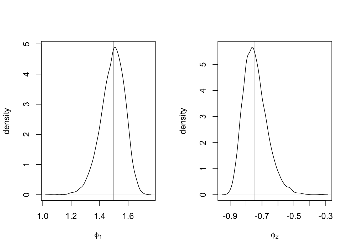

FIGURE 3.9: Marginal posterior densities of \(\phi_1\) (left panel) and \(\phi_2\) (right panel) in the AR(2) with level plus noise model. The vertical lines represent the true values assumed in the simulation.

Since R-INLA parametrizes \(\phi_1\) and \(\phi_2\) as \(r_1\) and \(r_2\) (see (3.9)), we show the code to obtain their marginal posteriors as well (see Figure 3.10).

par(mfrow = c(1, 2))
plot(
  model.ar2$marginals.hyperpar$`PACF1 for id.x`,
  type = "l",
  main = "",
  xlab = expression(r[1]),
  ylab = "density"
)
plot(
  model.ar2$marginals.hyperpar$`PACF2 for id.x`,
  type = "l",
  main = "",
  xlab = expression(r[2]),
  ylab = "density"
)

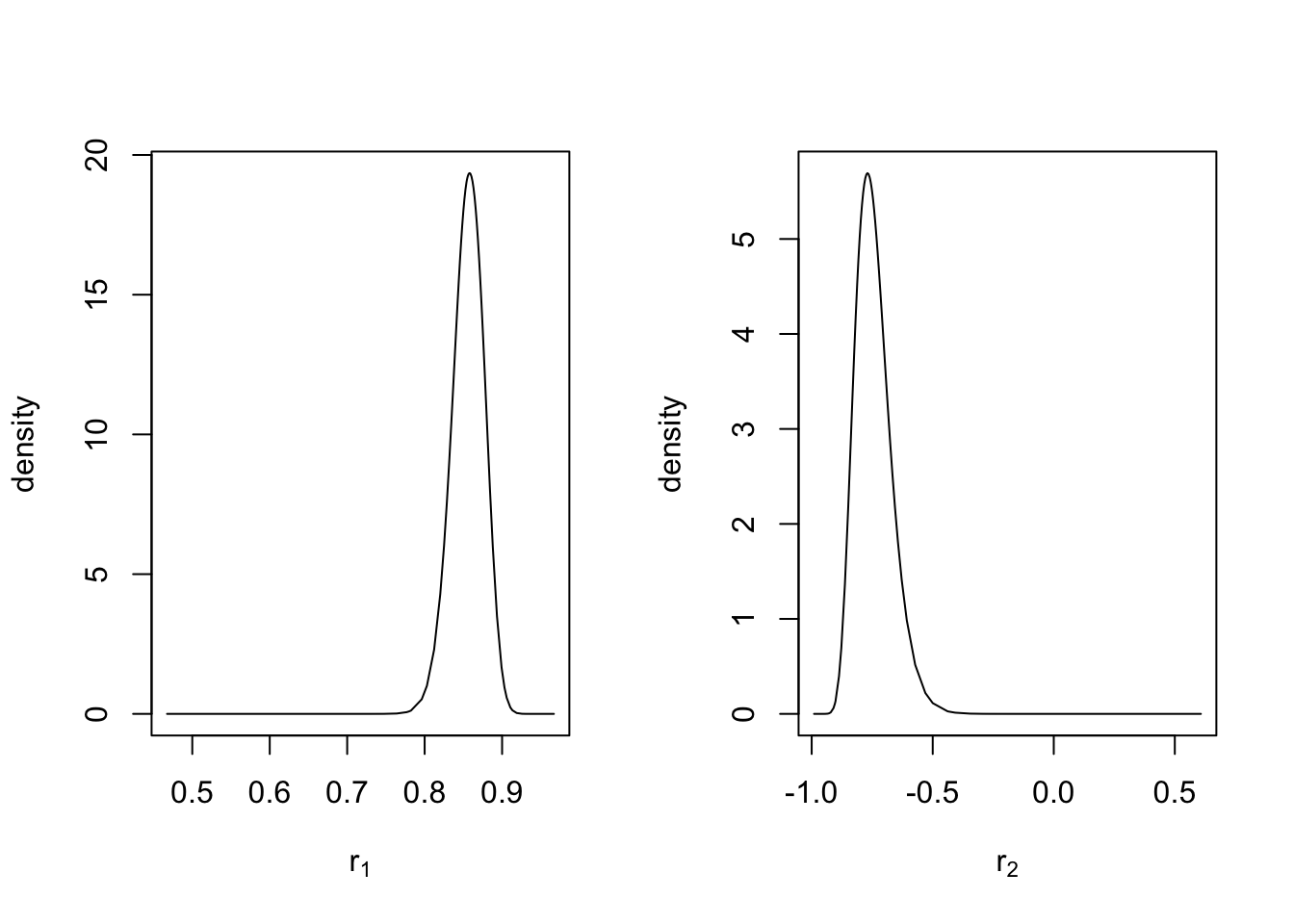
FIGURE 3.10: Marginal posterior densities of PACF(1) and PACF(2) in the internal R-INLA representation for an AR(2) with level plus noise model.

We end this section with a note that the syntax for fitting an AR\((p)\) model also works when \(p=1\), so that we can also fit an AR(1) with the level plus noise model using

formula <- y ~ f(id.x, model = "ar",order = 1) 

3.5 Random walk with drift plus noise model

The state equation describes \(x_t\) as a random walk with drift \(\delta\) plus Gaussian noise. We then observe the signal \(x_t\) with measurement noise, as described below:

\[\begin{align} y_t &= x_t + v_t;~~ v_t \sim N(0, \sigma^2_v), \tag{3.12}\\ x_t &= \delta + x_{t-1} + w_t;~~ w_t \sim N(0, \sigma^2_w). \tag{3.13} \end{align}\] Using the arima.sim() function, we simulate the latent Gaussian process \(x_t\), assuming a state error variance \(\sigma^2_w = 0.05\) and drift \(\delta = 0.1\). Adding Gaussian observation noise \(v_t\) with variance \(\sigma^2_v = 0.5\) then generates \(y_t\).

Since it is not possible to directly code the drift \(\delta\) into the R-INLA formula, we must reparameterize the model as follows. Let \(z_t\) denote a random walk process without drift, derived from the same Gaussian white noise \(w_t\). We can rewrite the random walk plus drift process \(x_t\) in (3.13) as

\[\begin{align} x_t &= \delta t + z_t, \\ z_t - z_{t-1} &= w_t, \tag{3.14} \end{align}\] so that

\[\begin{align*} x_t - x_{t-1} = \delta t + z_t - \delta (t-1) - z_{t-1}=\delta + (z_t - z_{t-1}) = \delta + w_t. \end{align*}\] Substituting \(x_t\) from (3.14) into the observation equation (3.12), we get the model

\[\begin{align} y_t &= \delta t + z_t + v_t;~~ v_t \sim N(0, \sigma^2_v), \tag{3.15} \\ z_t &= z_{t-1} + w_t;~~ w_t \sim N(0, \sigma^2_w). \tag{3.16} \end{align}\] That is, we have re-written a DLM with a drift coefficient in the state equation (see (3.13)) as a DLM with a deterministic trend \(\delta t\) in the observation equation (3.15), and a random walk without drift in the state equation (see (3.16)). This reparametrization of the DLM now enables us to formulate and fit the random walk with drift plus noise model in R-INLA. To illustrate, we generate a time series from this model; see Figure 3.11.

sim.rw1.drift <-
  simulation.from.rw1(
    sample.size = 500,
    burn.in = 100,
    level = 0,
    drift = 0.1,
    V = 0.5,
    W = 0.05,
    plot.data = TRUE,
    seed = 1
  )
sim.rw1.drift$sim.plot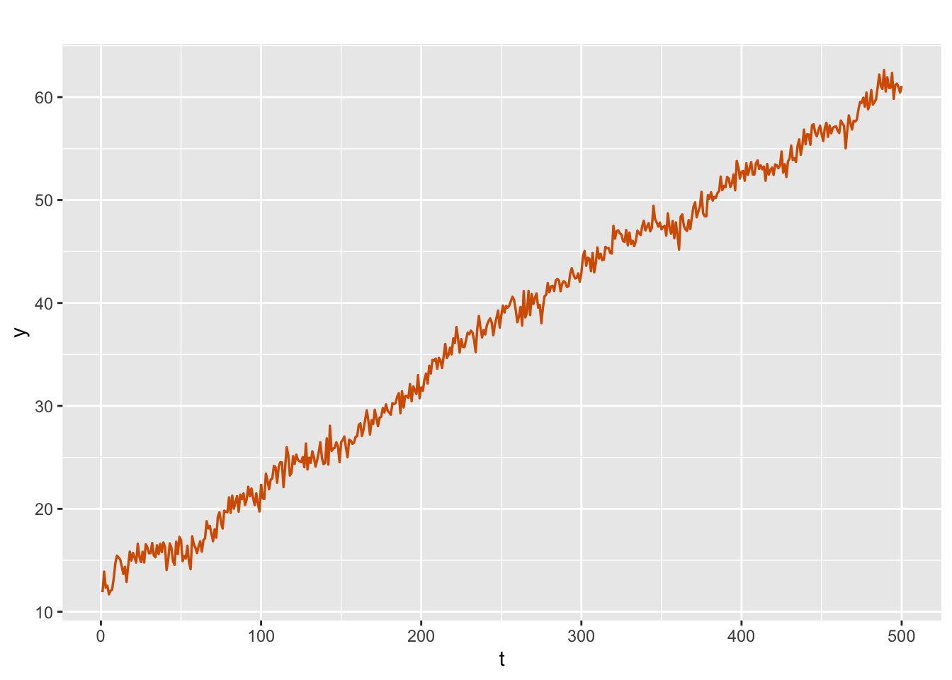

FIGURE 3.11: Simulated data from a random walk with drift plus noise model.

There are two ways to implement the modeling in R-INLA.

Method 1. Let id.delta correspond to the non time-varying coefficient \(\delta\) in (3.15), taking values from \(1\) to \(n\). Let id.w be an \(n\)-dimensional vector denoting the white noise \(w_t\) which corresponds to \(z_t\) (the random walk process without drift defined in (3.16)). We assume the prior distribution of \(\delta\) to be \(N({\rm mean} = 0, {\rm precision} = 0.001)\), the default prior specification, which is a vague prior specification on \(\delta\). This can be accessed from inla.set.control.fixed.default()[c("mean", "prec")]. The priors for \(\theta_v = \log(1/\sigma^2_v)\) and \(\theta_w = \log(1/\sigma^2_w)\) have been described earlier. Based on the time indexes id.w and id.delta, we create a data frame rw1.drift.dat with three columns containing the time series \(y_t\) and the time indexes. The formula, model setup, and results are shown below.

y.rw1.drift <- sim.rw1.drift$sim.data
n <- length(y.rw1.drift)
id.w <- id.delta <- 1:n
rw1.drift.dat <- cbind.data.frame(y.rw1.drift, id.w, id.delta)

formula.rw1.drift.1 <-
  y.rw1.drift ~ f(id.w, model = "rw1", constr = FALSE) - 1 + id.delta  
model.rw1.drift.1 <- inla(
  formula.rw1.drift.1,
  family = "gaussian",
  data = rw1.drift.dat,
  control.predictor = list(compute = TRUE)
)
# summary(model.rw1.drift.1)
format.inla.out(model.rw1.drift.1$summary.fixed[,c(1:5)])
##   name     mean  sd   0.025q 0.5q  0.975q
## 1 id.delta 0.098 0.01 0.079  0.098 0.117
format.inla.out(model.rw1.drift.1$summary.hyperpar[,c(1:2)])
##   name                       mean   sd   
## 1 Precision for Gaussian obs  1.717 0.125
## 2 Precision for id.w         23.676 5.893

From the output, we see that the posterior mean of \(\delta\) is 0.098 with a posterior standard deviation of 0.01; recall that the true value of \(\delta\) is \(0.1\). The estimates of \(\sigma^2_v\) and \(\sigma^2_w\) are respectively 0.582 (true value is \(0.5\)) and 0.042 (true value is \(0.05\)). Note that if we wish to change the prior specification on \(\delta\), we can use control.fixed within inla() (although we do not show this here).

prior.fixed <- list(mean = 0, prec = 0.1)
inla(formula = ,
     data = ,
     control.fixed = prior.fixed)

Method 2. This is an equivalent R-INLA approach for this model and uses a formulation with the model = linear option.

formula.rw1.drift.2 <-
  y.rw1.drift ~ f(id.w, model = "rw1", constr = FALSE) - 1 + 
  f(id.delta, model = "linear", mean.linear = 0, prec.linear = 0.001)
model.rw1.drift.2 <- inla(
  formula.rw1.drift.2,
  family = "gaussian",
  data = rw1.drift.dat,
  control.predictor = list(compute = TRUE)
)
# summary(model.rw1.drift.2)
format.inla.out(model.rw1.drift.2$summary.fixed[,c(1:5)])
##   name     mean  sd   0.025q 0.5q  0.975q
## 1 id.delta 0.098 0.01 0.079  0.098 0.117
format.inla.out(model.rw1.drift.2$summary.hyperpar[,c(1:2)])
##   name                       mean   sd   
## 1 Precision for Gaussian obs  1.717 0.125
## 2 Precision for id.w         23.676 5.893

Note that we get similar results from both methods, and we may use either code to fit and analyze this model. Similar to what we have seen earlier, the following code is useful to recover and print posterior estimates of \(\sigma^2_v\), \(\sigma^2_w\) and \(\delta\) from the inla() output.

sigma2.v.hat <-
  inla.emarginal(
    fun = function(x)
      exp(-x),
    marginal = model.rw1.drift.1$internal.marginals.hyperpar$
      `Log precision for the Gaussian observations`
  )
sigma2.w.hat <-
  inla.emarginal(
    fun = function(x)
      exp(-x),
    marginal = model.rw1.drift.1$internal.marginals.hyperpar$
      `Log precision for id.w`
  )
cat(paste(
  "Estimated observation noise variance, sigma2.v",
  round(sigma2.v.hat, 2),
  sep = " = "
),
"\n")
## Estimated observation noise variance, sigma2.v = 0.59
cat(paste(
  "Estimated state noise variance, sigma2.w",
  round(sigma2.w.hat, 2),
  sep = " = "
),
"\n")
## Estimated state noise variance, sigma2.w = 0.04
delta.hat <- model.rw1.drift.1$summary.fixed$mean
cat(paste("Estimated drift, delta", round(delta.hat, 2), sep = " = "), "\n")
## Estimated drift, delta = 0.1

Also, as we discussed earlier, we can pull out the posterior distributions of the hyperparameters using inla.tmarginal() and obtain HPD intervals using inla.hpdmarginal() (code not shown here). We will revisit Method 2 in Chapter 5, further explaining the available options related to the term linear in the formula. We next describe an approach to use R-INLA for modeling a DLM with a time-varying drift in the state equation.

3.6 Second-order polynomial model

Given an observed time series \(y_t,~t=1,\ldots,n\), consider the model with a random walk latent state \(x_t\) with a random, time-varying drift \(\delta_{t-1}\):

\[\begin{align} y_t&= x_t + v_t, \tag{3.17} \\ x_t &= x_{t-1}+\delta_{t-1}+w_{t,1}, \tag{3.18}\\ \delta_{t} &= \delta_{t-1} + w_{t,2}. \tag{3.19} \end{align}\] This is usually called the second-order polynomial model. Similar models have been discussed in Ruiz-Cárdenas, Krainski, and Rue (2012).

Let \({\boldsymbol x}^\ast_t = (x_t, \delta_t)'\) be the \(2\)-dimensional state vector with \(x^\ast_{t,1} =x_t\) and \(x^\ast_{t,2}=\delta_t\). For \(t=2,\ldots,n\), we can write (3.18) and (3.19) as

\[\begin{align} {\boldsymbol x}^\ast_t &= \begin{pmatrix} 1 & 1 \\0 & 1 \end{pmatrix} {\boldsymbol x}^\ast_{t-1} + {\boldsymbol w}^\ast_t \notag \\ &= \boldsymbol{\Phi} {\boldsymbol x}^\ast_{t-1} + {\boldsymbol w}^\ast_t, \text{ say}, \tag{3.20} \end{align}\] where \(\boldsymbol{\Phi} = \begin{pmatrix} 1 & 1 \\0 & 1 \end{pmatrix}\) is a \(2 \times 2\) state transition matrix. We assume that \({\boldsymbol w}^\ast_t \sim N({\boldsymbol 0},{\boldsymbol W})\), where \({\boldsymbol W} =\text{diag}(\sigma^2_{w1},\sigma^2_{w2})\). The observation equation in the model is a linear function of the bivariate state vector \({\boldsymbol x}^\ast_t\) plus an observation noise \(v_t\):

\[\begin{align} y_t = (1, \ 0) {\boldsymbol x}^\ast_t + v_t, \ t=1,\ldots,n, \tag{3.21} \end{align}\] where \(v_t \sim N(0, V)\).

Following Ruiz-Cárdenas, Krainski, and Rue (2012), we can express (3.20) as

\[\begin{align} {\boldsymbol 0} = {\boldsymbol x}^\ast_t - \boldsymbol{\Phi} {\boldsymbol x}^\ast_{t-1} - {\boldsymbol w}^\ast_t, \ t=2,\ldots,n, \tag{3.22} \end{align}\] yielding a set of \(n-1\) faked zero observations on the left side written as a linear function of the terms on the right side. That is, we rewrite the state equations (3.18) and (3.19) as

\[\begin{align} 0 &= x_t - x_{t-1} -\delta_{t-1} - w_{t,1}, \tag{3.23}\\ 0 &= \delta_{t} - \delta_{t-1} - w_{t,2}. \tag{3.24} \end{align}\]

Then, the augmented model has dimension \(n+ 2(n-1)\), the \(n\) observations \(y_1,\ldots,y_n\) being stacked together with the set of \(n-1\) faked zero observations in (3.22):

\[\begin{align} \begin{pmatrix} y_1 & NA & NA \\ \vdots & \vdots & \vdots \\ y_n & NA & NA \\ \hline \\ NA & 0 & NA \\ \vdots & \vdots & \vdots \\ NA & 0 & NA \\ \hline \\ NA & NA & 0 \\ \vdots & \vdots & \vdots \\ NA & NA & 0 \end{pmatrix}, \tag{3.25} \end{align}\] where each of the second and third horizontal blocks has dimension \((n-1) \times 3\). The first \(n\) rows of Column 1 contain the observations, \(y_1,\ldots,y_n\). Column 2 is associated with the first state variable \(x^\ast_{t,1}=x_t\) whose entries are forced to zero for \(t=2,\ldots,n\) (see (3.22)). Column 3 is associated with the second state variable \(x^\ast_{t,2}=\delta_t\) for \(t=2,\ldots,n\). All the other entries in the structure have no values and are assigned NAs. In summary, this augmented structure in (3.25) will have the observed \(y_t\) in the first \(n\) rows of Column 1, and there will be as many additional columns as the number of state variables in the state equation (here, \(2\)).

For fitting the model, R-INLA considers different likelihoods for Column 1 and the other columns of the augmented structure in (3.25). As described in Ruiz-Cárdenas, Krainski, and Rue (2012), given the state vector \({\boldsymbol x}^\ast_t\), the data \(y_t,~t=1,\ldots,n\) are assumed to follow a Gaussian distribution with unknown precision \(V^{-1}\). Given \({\boldsymbol x}^\ast_t, {\boldsymbol x}^\ast_{t-1}\) and \({\boldsymbol w}^\ast_t\), the faked zero data in Columns 2 and 3 of (3.25) are artificial observations and are assumed to be deterministic (i.e., known, with zero variance). R-INLA represents this condition by assuming that these faked zero data follow a Gaussian distribution with a high, fixed precision. It is assumed that for \(t = 1\), \({\boldsymbol x}^\ast_1\) follows a noninformative distribution, i.e., a bivariate normal distribution with a fixed and low-valued precision matrix. For \(t = 2,\ldots,n\), it is assumed that \({\boldsymbol x}^\ast_t\) follows (3.20) and \({\boldsymbol w}^\ast_t \sim N({\boldsymbol 0},{\boldsymbol W})\):

\[\begin{align*} f_{{\boldsymbol w}^\ast_t}({\boldsymbol x}^\ast_t - \boldsymbol{\Phi}{\boldsymbol x}^\ast_{t-1}) \propto \exp[-\frac{1}{2} ({\boldsymbol x}^\ast_t - \boldsymbol{\Phi}{\boldsymbol x}^\ast_{t-1})'{\boldsymbol W}^{-1}({\boldsymbol x}^\ast_t - \boldsymbol{\Phi}{\boldsymbol x}^\ast_{t-1})]. \end{align*}\] We must define the \(n \times 2\) matrix \({\boldsymbol X}^\ast =({\boldsymbol x}^\ast_1, \ldots,{\boldsymbol x}^\ast_n)'\), and also define \({\boldsymbol X}^\ast_{(-1)} =({\boldsymbol x}^\ast_2, \ldots,{\boldsymbol x}^\ast_n)'\) and \({\boldsymbol X}^\ast_{(-n)} =({\boldsymbol x}^\ast_1, \ldots,{\boldsymbol x}^\ast_{n-1})'\).

The following code simulates a time series \(y_t\), see Figure 3.12, of length \(n=200\). The true values of the error variances are assumed to be \(V = 0.01\), and \({\boldsymbol W} = \text{diag}(0.0001, 0.0001)\).

sim.secondorder <-
  simulation.from.second.order.dlm(
    sample.size = 200,
    V = 0.01,
    W1 = 1e-04,
    W2 = 1e-04,
    plot.data = TRUE,
    seed = 123457
  )
sim.secondorder$sim.plot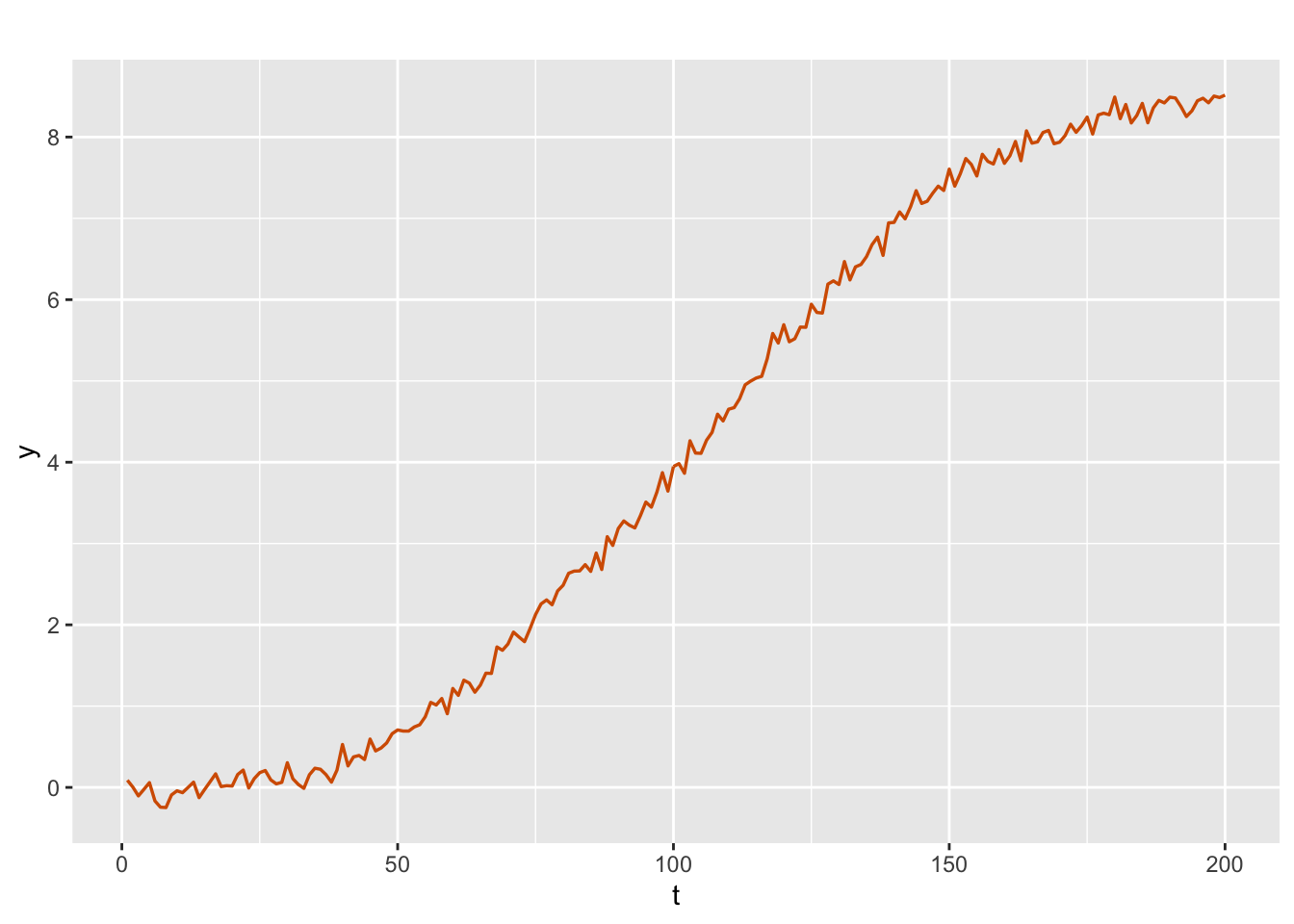

FIGURE 3.12: Simulated data from a second-order polynomial model.

y.sec <- sim.secondorder$sim.data
n <- length(y.sec)

The following code sets up the augmented model. Let \(m = n-1\). The observed time series \(y_t\) forms the first block of rows.

m <- n-1
Y <- matrix(NA, n+2*m, 3)
# actual observations (y.sec)
Y[1:n, 1] <- y.sec 
Y[1:m + n, 2] <- 0  
Y[1:m + (n+m), 3] <- 0  

The set up of the vectors of indexes and vectors of weights (coefficients) for the different latent variables follows the discussion in Ruiz-Cárdenas, Krainski, and Rue (2012) (also see their Appendix). In order to avoid confusion with the state errors \(w_t\), we use the symbols \(\boldsymbol{ci}, \boldsymbol{cj}\), etc., instead of \(\boldsymbol{wi}, \boldsymbol{wj}\), etc., to denote the weights (coefficients). We give a description of these items for this model.

1. The vector of indexes denoted by \({\boldsymbol i}\) for the latent series \(x^\ast_{t,1} =x_t\) consists of (a) a vector \(c(1:n)\) of length \(n\) (from the observation equation), (b) a vector \(c(2:n)\) of length \(m\) (from the rewritten first state equation (3.23) for \(x^\ast_{t,1}=x_t\) with fake zeroes), and (c) a vector of NA’s of length \(m\) (from the rewritten second state equation (3.24) for \(x^\ast_{t,2}=\delta_t\) with fake zeroes).

2. The vector of indexes \({\boldsymbol j}\) for the latent series \(x^\ast_{t-1,1}=x_{t-1}\) consists of (a) a vector of NA’s of length \(n\) (since the observation equation has no \(x_{t-1}\)), (b) a vector \(c(1:m)\) of length \(m\) (from the rewritten state equation (3.23)), and (c) a vector of NA’s of length \(m\) (since the rewritten second state equation (3.24) has no \(x_{t-1}\)).

3. The vector \(\boldsymbol{cj}\) consists of the coefficients corresponding to the vector \(\boldsymbol{j}\) and has (a) a vector of NA’s of length \(n\) (since the observation equation has no \(x_{t-1}\)), (b) a vector of length \(m\) with elements \(-1\) (corresponding to the coefficient of \(x_{t-1}\) in (3.23)), and (c) a vector of NA’s of length \(m\) (since the second state equation has no \(x_{t-1}\)).

4. The vector of indexes \(\boldsymbol{l}\) for the latent series \(x^\ast_{t,2}=\delta_t\) consists of (a) a vector of NA’s of length \(n\) (since the observation equation has no \(\delta_{t}\)), (b) a vector of NA’s of length \(m\) (since the first state equation has no \(\delta_{t}\)), and (c) a vector \(c(2:n)\) of length \(m\) (corresponding to the coefficient of \(\delta_{t}\) in the rewritten second state equation).

5. The vector \(\boldsymbol{cl}\) consists of coefficients corresponding to the vector \(\boldsymbol{l}\) and has (a) a vector of NA’s of length \(n\) (since the observation equation has no \(\delta_{t}\)), (b) a vector of NA’s of length \(m-1\) (since the first rewritten state equation (3.23) has no \(\delta_{t}\)), and (c) a vector of length \(m\) with elements 1 (corresponding to the coefficient of \(\delta_t\) in (3.24)).

6. The vector of indexes \(\boldsymbol{k}\) for the latent series \(x^\ast_{t-1,2}=\delta_{t-1}\) consists of (a) a vector of NA’s of length \(n\) (since the observation equation has no \(\delta_{t-1}\)), (b) a vector \(c(1:m)\) of length \(m\) (from the rewritten state equation (3.23)), and (c) a vector \(c(1:m)\) of length \(m\) (from the rewritten state equation (3.23)).

7. The vector \(\boldsymbol{ck}\) consists of coefficients corresponding to the vector of indexes \(\boldsymbol{k}\) and has (a) a vector of NA’s of length \(n\) (since the observation equation has no \(\delta_{t-1}\)), (b) a vector of length \(m\) with elements \(-1\) (corresponding to the coefficient of \(\delta_{t-1}\) in (3.23)), and (c) a vector of length \(m\) with elements \(-1\) (corresponding to the coefficient of \(\delta_{t-1}\) in (3.24)).

8. The vector \(\boldsymbol{q}\) consists of indexes for the state errors (perturbations) \(w_{t,1}\) in (3.23) and has NA’s in all entries except for the \(m\) middle entries corresponding to (3.23).

9. The vector \(\boldsymbol{cq}\) correspondingly has \(-1\) in the middle \(m\) positions and NA’s otherwise.

10. The vector \(\boldsymbol{s}\) consists of indexes for the state errors (perturbations) \(w_{t,2}\) in (3.24) and has NA’s in all entries except for the last \(m\) entries corresponding to (3.24).

11. The vector \(\boldsymbol{cs}\) correspondingly has \(-1\) in the last \(m\) positions and NA’s otherwise.

i <- c(1:n, 2:n, rep(NA, m))              # indexes for x_t
j <- c(rep(NA, n), 2:n - 1, rep(NA, m))     # indexes for x_{t-1}
cj <- c(rep(NA, n), rep(-1, m), rep(NA, m)) # weights for x_{t-1}
l <- c(rep(NA, n + n - 1), 2:n)         # indexes for delta_t
cl <- c(rep(NA, n + m), rep(1, m))      # weights for delta_t
k <- c(rep(NA, n), 2:n - 1, 2:n - 1)  # indexes for delta_{t-1}
ck <- c(rep(NA, n), rep(-1, 2 * m))     # weights for delta_{t-1}
q <- c(rep(NA, n), 1:m, rep(NA, m))  # indexes for w_{t,1}
s <- c(rep(NA, n + m), 1:m)           # indexes for  w_{t,2}
cq <- c(rep(NA, n), rep(-1, m), rep(NA, m)) # weights for w_{t,1}
cs <- c(rep(NA, n + m), rep(-1, m))          # weights for w_{t,2}

The model formulation is shown below. The first term handles the first state variable \(x_t\) (with index vector \({\boldsymbol i}\)) while the second term handles the state variable \(x_{t-1}\) (with index vector \({\boldsymbol j}\)). Since both have the same distribution, we may use f(j, wj, copy="i"). A similar usage follows for index vectors \(\boldsymbol l\) and \(\boldsymbol k\) for the second state variables \(\delta_t\) and \(\delta_{t-1}\). The R-INLA feature copy enables us to share terms among different parts of the model and is explained below (also see Section 6.5 of Gómez-Rubio (2020)).

R-INLA feature copy

Using the copy feature when defining different likelihoods associated with different latent random variables allows us to ensure that linear predictors of the different likelihoods share the same type of latent effect, with the values of the random effects being the same, while copied effects can be scaled by a parameter. All copies of the random effects share the same hyperparameters.

formula.second.poly = Y ~ f(i, model="iid", initial=-10, fixed=TRUE) +
              f(j, cj, copy="i") + 
            f(l, cl, model="iid", values = 1:n, initial=-10, fixed=TRUE)+
              f(k, ck, copy="l")+
              f(q, cq, model ="iid") + 
              f(s, cs, model ="iid") -1

Here, \(\boldsymbol i\) is the index variable used in the original effect, i.e., \(x_t\), and \(\boldsymbol j\) is the index corresponding to \(x_{t-1}\) which must take values in the same set as \(\boldsymbol i\). In general, the new index \(\boldsymbol j\) need not have the same ordering as \(\boldsymbol i\), and only the elements of \(x_t\) that are indexed in \(\boldsymbol j\) will be copied (as pointed out in Gómez-Rubio (2020)).

The argument values in the function f()is used to provide the set of all values assumed by the covariate for which we want the estimated effect. By default, values assumes the unique set of values defined in the index; for example, for index \(\boldsymbol l\), the set is \(\{2,\ldots,n\}\). In the model formula for the index \(\boldsymbol k\), we have \(copy =``\text{l}"\); the argument copy enables the index \(\boldsymbol k\) to inherit values of the argument values defined for index \(\boldsymbol l\). However, note that values for \(f(k, ck, copy= ``\text{l}")\) is the set \(\{1,\ldots,n-1\}\). Therefore, for inla() to run without error, it is necessary to inform the model that \(\boldsymbol l\) is being copied, for which we must include values = 1:n in the function f() defined for \(\boldsymbol l\).

model.second.poly = inla(
  formula.second.poly,
  data = data.frame(i, j, cj, k, ck, l, q, s, cq, cs),
  family = rep("gaussian", 3),
  control.family = list(
    list(),
    list(initial = 10, fixed = TRUE),
    list(initial = 10, fixed = TRUE)
  ),
  control.predictor = list(compute = TRUE)
)
format.inla.out(model.second.poly$summary.hyperpar[,c(1:2)])
##   name                       mean  sd      
## 1 Precision for Gaussian obs   105    11.25
## 2 Precision for q            20081 16381.84
## 3 Precision for s            51361 26504.35

post.mean.V <- inla.emarginal(
  fun = function(x)
    exp(-x),
  marginal = model.second.poly$internal.marginals.hyperpar$
    `Log precision for the Gaussian observations`
)
post.mean.W11 <- inla.emarginal(
  fun = function(x)
    exp(-x),
  marginal = model.second.poly$internal.marginals.hyperpar$
    `Log precision for s`
)
post.mean.W22 <- inla.emarginal(
  fun = function(x)
    exp(-x),
  marginal = model.second.poly$internal.marginals.hyperpar$
    `Log precision for q`
)

The posterior mean of \(V\) is 0.0096. The posterior means of \(\sigma^2_{w1}\) and \(\sigma^2_{w2}\) are 0.000025 and 0.00009833 respectively, and are not recovered as accurately as the mean of \(V\).

3.7 Forecasting states and observations

An important goal in time series analysis is to forecast future values of a time series based on a fitted model. Suppose we split the observed data into a fitting or training portion \(y_1,\ldots, y_{n_t}\) and a holdout or test portion \(y_{n_t +1},\ldots, y_{n_t + n_h}\). The training portion is of length \(n_t\), and the holdout portion is of length \(n_h\). In the Bayesian DLM framework, given the training data \(y_1,\ldots, y_{n_t}\), estimates of the states \(x_1,\ldots, x_{n_t}\) and estimates of the model hyperparameters \(\boldsymbol{\theta}\), we first forecast \(x_{n_t+\ell},~\ell=1,\ldots,n_h\) by \(f(x_{n_t+\ell}|\boldsymbol{y}^n),~\ell=1,\ldots,n_h\). We then obtain \(n_h\) forecasts of \(y_{n_t+\ell}\) by \(f(y_{n_t+\ell}|\boldsymbol{y}^n),~\ell=1,\ldots,n_h\).

In R-INLA, there is no separate forecasting function like the predict() function in the stats package which is commonly used with functions such as lm(). Therefore, we append the end of the training data of length \(n_t\) with NA’s to represent the times to hold out the last \(n_h\) data points. Forecasts for \(x_{n_t+\ell}\) are obtained using the summary.random option. For example, we can forecast \(n_h = 10\) future states in the AR(1) with level plus noise model; we use the summary.random option, as shown below.

format.inla.out(tail(model.ar1.level$summary.random$id.x[,c(1:3)],10))
##    ID  mean   sd   
## 1  491  0.105 0.272
## 2  492 -0.169 0.273
## 3  493 -0.437 0.300
## 4  494 -0.135 0.273
## 5  495  0.220 0.279
## 6  496  0.239 0.275
## 7  497  0.122 0.272
## 8  498  0.295 0.276
## 9  499  0.261 0.275
## 10 500  0.259 0.281

We then obtain \(n_h =10\) future forecasts \(y_{n_t+\ell}\) using

format.inla.out(tail(model.ar1.level$summary.fitted.values[,c(1:3)],10))
##    name         mean  sd    0.025q
## 1  fit.Pred.491 1.392 0.271 0.864 
## 2  fit.Pred.492 1.118 0.273 0.575 
## 3  fit.Pred.493 0.850 0.300 0.243 
## 4  fit.Pred.494 1.152 0.272 0.611 
## 5  fit.Pred.495 1.507 0.278 0.972 
## 6  fit.Pred.496 1.526 0.275 0.996 
## 7  fit.Pred.497 1.409 0.272 0.872 
## 8  fit.Pred.498 1.583 0.276 1.050 
## 9  fit.Pred.499 1.549 0.274 1.016 
## 10 fit.Pred.500 1.547 0.281 1.002

Figure 3.13 shows the time series generated by the AR(1) with level plus noise model, together with the last \(10\) forecasts. For a better visualization of forecasts (means of the posterior predictive distributions) and 2 standard deviation bounds, we show a plot with only the last 100 data points.

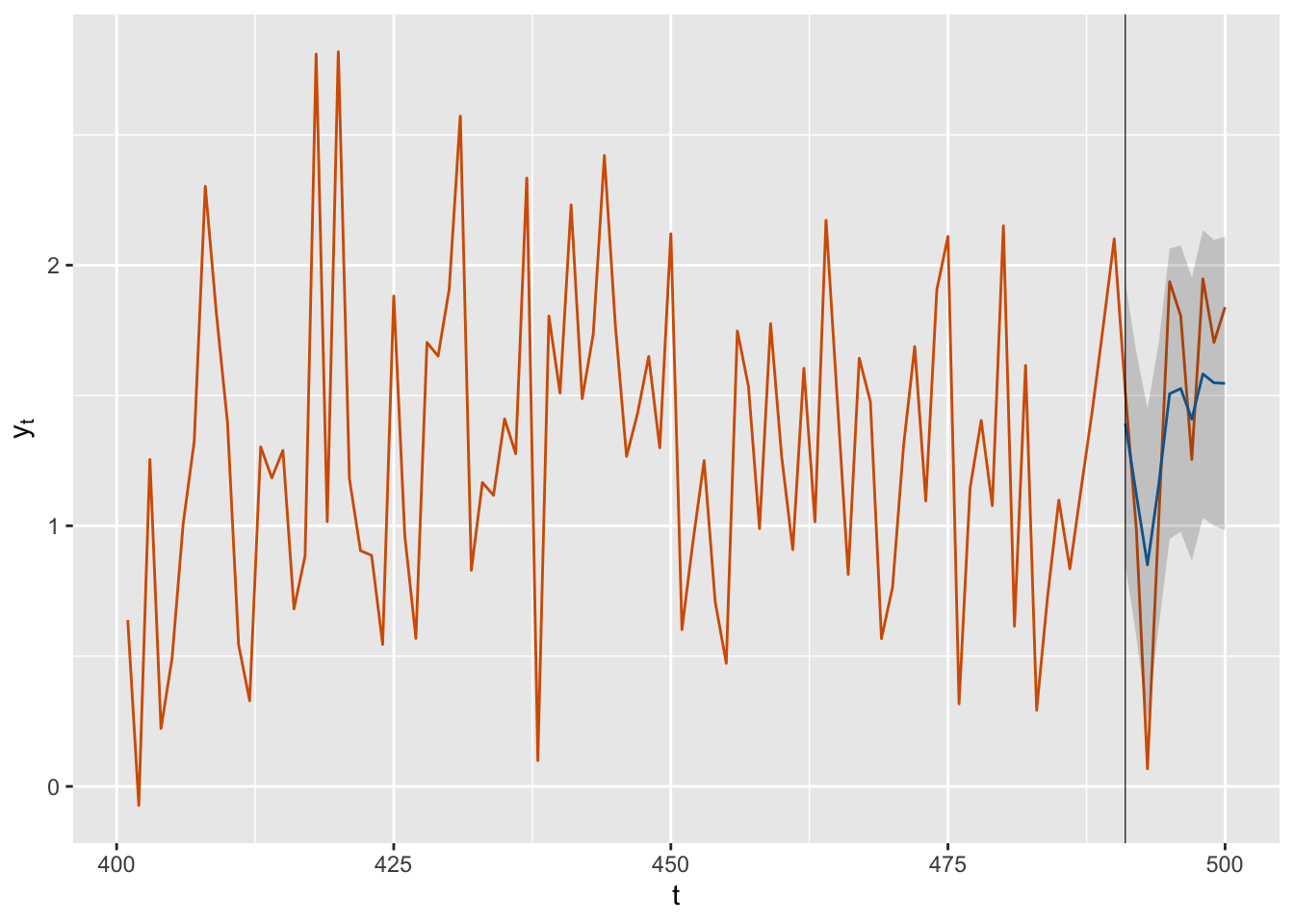
FIGURE 3.13: Forecasts (blue) for ten future time points along with observed data (red) from the AR(1) with level plus noise model. The black vertical line divides the data into training and test portions. The gray shaded area shows forecast intervals based on 2 standard deviation (sd) bounds around the means of the posterior predictive distributions.

3.8 Model comparisons

In this section, we explain how to compare different fitted models. Many model comparison criteria have been defined in the Bayesian framework, including the conditional predictive ordinate (CPO), the Bayes factor (BF), the deviance information criterion (DIC), and the Watanabe Akaike information criterion (WAIC). These are useful for comparing the relative performance of the fitted models based on the calibration (or training or fitting) data, and were reviewed in Chapters 1 and 2. We may also compare models based on their predictive performance using frequentist metrics such as the mean absolute percent error (MAPE) or mean absolute error (MAE). These two metrics can be computed from in-sample training data as well as out-of-sample test data.

3.8.1 In-sample model comparisons

We start with a discussion of in-sample model comparisons and illustrate code for the random walk plus noise model. In R-INLA, we compute these quantities using the control.compute option in the formula. If the output is saved in out, we can access the predictive quantities as out$dic$dic, or out$cpo$cpo, or out$cpo$pit, as shown below.

1. The deviance information criterion (DIC) was defined in (1.9). We use the control.compute option to obtain the DIC, via control.compute=list(dic=TRUE), and access it by out$dic$dic.

model.rw1 <- inla(
  formula.rw1,
  family = "gaussian",
  data = rw1.dat,
  control.predictor = list(compute = TRUE),
  control.compute = list(dic = TRUE, cpo = TRUE)
)
model.rw1$dic$dic
## [1] 1312

2. The conditional predictive ordinate (CPO) was defined in Chapter 1 as \(p(y_t \vert \boldsymbol y_{(-t)})\), a “leave-one-out” measure of model fit. The sum of the log CPO values gives us the pseudo-Bayes factor. We again use control.compute=list(cpo=TRUE), and access it by out$cpo$cpo.

cpo.rw1 <- model.rw1$cpo$cpo
psBF.rw1 <- sum(log(cpo.rw1))
psBF.rw1
## [1] -671

3. The probability integral transform (PIT) defined by

\[\begin{align} p(y_t^{\mbox{new}} \le y_t \vert \boldsymbol y_{(-t)}) \tag{3.26} \end{align}\] is another “leave-one-out” measure of fit computed by R-INLA. A histogram of PIT must resemble a uniform distribution; extreme values indicate outlying observations. We again use control.compute=list(cpo=TRUE), and access by using out$cpo$pit. The plot in Figure 3.14 gives an indication of model adequacy, since the histogram is close to that of a sample from a uniform distribution.

pit.rw1 <- model.rw1$cpo$pit
hist(pit.rw1,main =" ", ylab="frequency")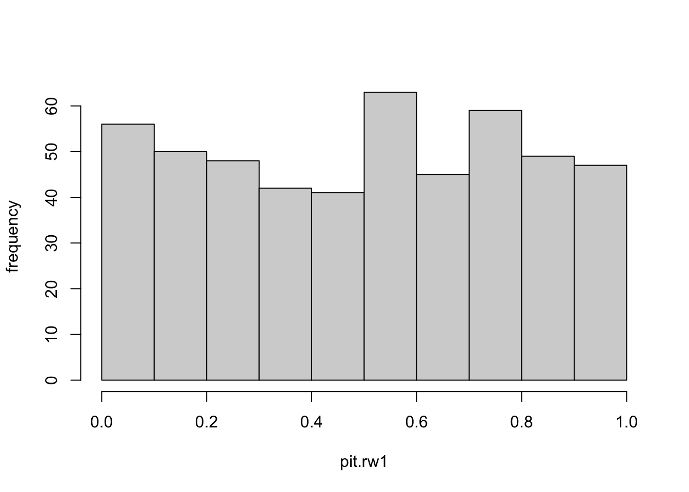

FIGURE 3.14: Histogram of the probability integral transform (PIT) for the random walk plus noise model.

Note that R-INLA computes CPO or PIT by keeping the integration-points fixed. To get improved grid integration, we can include, for instance, control.inla=list(int.strategy = "grid", diff.logdens = 4). Also, to increase the accuracy of the tails of the marginals, we can use control.inla = list(strategy = "laplace", npoints = 21). This adds 21 evaluation points instead of the default npoints=9.

It is useful to understand what the following check for failure means. R-INLA makes some implicit assumptions which are tested using internal checks. If model.rw1$cpo$failure[i] == 0, then no assumption is violated. If model.rw1$cpo$failure[i] > 0 for any row \(i\) of the data, this indicates that some assumption is violated, larger values (maximum value is \(1\)) indicating more serious violations of assumptions.

table(model.rw1$cpo$failure)
## 
##   0 
## 500

It might be a good idea to recompute those, if any, CPO/PIT values for which result$cpo$failure>0. INLA has provided improved.result = inla.cpo(result). This takes an object which is the output from inla(), and recomputes (in an efficient way) the CPO/PIT for which result$cpo$failure > 0, and returns model.rw1 with the improved estimates of CPO/PIT. See ?inla.cpo for details. R-INLA recommends caution when using CPO or PIT for model validation, since they may depend on tail behavior, which is difficult to estimate. We can verify that the smallest CPO values are estimated correctly by setting res$cpo$failure[smallest cpo indices] = 1 and re-estimating them with inla.cpo().

4. R-INLA also outputs the marginal likelihood (see the definition in Chapter 1) on the logarithmic scale by default. Recall that a model with higher marginal likelihood is preferred.

model.rw1$mlik
##                                         [,1]
## log marginal-likelihood (integration) -750.0
## log marginal-likelihood (Gaussian)    -750.3

3.8.2 Out-of-sample comparisons

Let \(y_{n_t} (\ell)\) denote the forecast from origin \(n_t\) for \(y_{t+\ell},~\ell=1,\ldots,n_h\), and let \(e_{n_t} (\ell) = y_{n_t+\ell} - y_{n_t} (\ell)\) be the \(\ell\)th forecast error. The mean absolute percent error (MAPE) is a well known criterion, defined by

\[\begin{align} {\rm MAPE} = \frac{100}{n_h} \sum_{\ell=1}^{n_h}\vert e_{n_t}(\ell)/y_{n_t+\ell}\vert. \tag{3.27} \end{align}\] Another widely used criterion is the mean absolute error (MAE) given by

\[\begin{align} {\rm MAE} = \frac{1}{n_h} \sum_{\ell=1}^{n_h} |e_{n_t}(\ell)|. \tag{3.28} \end{align}\] Small values of MAPE and MAE indicate better fitting models. We show the custom code for computing MAPE and MAE in Chapter 14. We can also compute in-sample MAPE and in-sample MAE, as we discuss in the following chapters.

3.9 Non-default prior specifications

We look at a few ways for specifying non-default priors for hyperparameters. A listing of all prior distributions that R-INLA supports is given in Table 14.4; this is similar to Table 5.2 in Gómez-Rubio (2020). In some situations, we may wish to use alternatives to the default prior specifications, selecting one of the other options available in R-INLA. We show this using \(\theta_1 = \log(1/\sigma^2_w)\) and \(\theta_2 = \log(\frac{1+\phi}{1-\phi})\).

1. We can change the hyperprior parameter values from their default settings. For example, for the log-gamma prior for \(\log(1/\sigma^2_w)\), we can change param = c(1, 0.00005) to param = c(1, 0.0001) and/or initial = 4 to initial = 2. The prior for \(\theta_2\) will remain at its default setting.

hyper.state = list(
  theta1 = list(
    prior = "loggamma",
    param = c(1, 0.00005),
    initial = 4,
    fixed = FALSE
  )
)

2. Or, we may use other prior distributions, such as the beta correlation prior for \(\theta_2\) (see inla.doc("betacorrelation") for more details on this prior). The prior for \(\theta_1\) will remain at its default setting.

hyper.state = list(
  theta2 = list(
    prior = "betacorrelation",
    param = c(2, 2),
    initial = -1.098,
    fixed = FALSE
  )
)

The betacorrelation prior is a prior for the AR(1) correlation parameter \(\phi\) (recall this is denoted by \(\rho\) in R-INLA), represented internally as

\[\begin{align} \theta_{\phi,bc} = \log \frac{1+\phi}{1-\phi}. \tag{3.29} \end{align}\] This prior is defined on \(\theta_{\phi,bc}\) so that \(\phi\) is scaled to be in \((-1,1)\) and follow a Beta\((a,b)\) distribution given by

\[\begin{align*} \pi(\phi; a,b) = \frac{1}{2} \frac{\Gamma(a+b)}{\Gamma(a) \Gamma(b)} \phi^{a-1} (1-\phi)^{b-1}. \end{align*}\] The inverse transformation from \(\theta_{\phi,bc}\) to \(\phi\) is the same as for the default prior on \(\phi\), and is done by R-INLA, so that the output is provided on \(\phi\).

3.9.1 Custom prior specifications

In some examples, we may wish to specify priors that are not included in the list of priors provided in R-INLA and listed in names(inla.models()$prior). In such cases, there are two ways for building user-defined priors, i.e., table priors, which are based on tabulated values from the desired densities and expression priors, which are specified by formulas for the desired prior density functions.

Table Priors

The user provides a table with values of the hyperparameter defined on R-INLA’s internal scale and the associated prior densities on the log-scale. Values not defined in the table are interpolated at run time. INLA fits a spline through the points and continues with this in the succeeding computations. There is no transformation into a functional form. The input-format for the table is a string, which starts with table: and is then followed by a block of \(x\)-values and a block of corresponding \(y\)-values, which represent the values of the log-density evaluated at \(x\). The syntax is:

    table: x_1 ... x_n y_1 ... y_n

For more details, see inla.doc(“table”). As an example, suppose we wish to set up a Gaussian prior with zero mean and precision \(0.001\) for a hyperparameter \(\theta\) (on the internal scale). The following code sets this up as a table prior.

theta <- seq(-100, 100, by = 0.1)
log_dens <- dnorm(theta, 0, sqrt(1 / 0.001), log = TRUE)
gauss.prior <- paste0("table: ",
                      paste(c(theta, log_dens), collapse = " ")
)

Depending on what \(\theta\) represents, gauss.prior will be included either in formula under f() or in control.family, as mentioned earlier.

Expression Priors

The expression prior definition uses the muparser library.³ To set up a N\((0,0.01)\) prior on a hyperparameter \(\theta\) (i.e., with precision \(100\)), we can include the following code in the formula and model execution:

gauss.pr.e <- "expression:
  mean = 0;
  prec = 1000;
  logdens = 0.5 * log(prec) - 0.5 * log (2 * pi);
  logdens = logdens - 0.5 * prec * (theta - mean)^2;
  return(logdens);
"

R-INLA recognizes several well known functions that can be used within the expression statement. These include common mathematical functions, such as \(\exp(x)\), \(\sin(x)\), \(x^y\), \(\mbox{pow}(x;y)\) (to denote \(x\) raised to power \(y\)), \(\mbox{gamma}(x)\) and \(\mbox{lgamma}(x)\) (to denote the gamma function and its logarithm), etc.

3.9.2 Penalized complexity (PC) priors

R-INLA provides a useful framework for building penalized complexity (PC) priors (Fuglstad et al. 2019). These priors are defined on individual model components that can be regarded as flexible extensions of a simple and interpretable base model, and then penalizes deviations from the base model. This allows us to control flexibility, reduce over-fitting, and improve predictive performance. PC priors include a single parameter to control the degree of flexibility allowed in the model. They are specified by setting values \((U,\alpha)\) such that \(P(T(\xi) > U)=\alpha\), where \(T(\xi)\) is an interpretable transformation of the flexibility parameter \(xi\), and \(U\) is an upper bound that specifies a tail event with probability \(\alpha\).

For example, recall that we assumed an inverse log-Gamma prior on \(\sigma^2_v\). Instead, we can set a PC prior on the standard deviation \(\sigma_v\) by \(P(\sigma_v>1)=0.01\):

prior.prec <- list(prec = list(prior = "pc.prec",
                               param = c(1, 0.01)))

Documentation and details on the PC prior pc.prec can be seen in inla.doc("pc.prec").

3.10 Posterior sampling of latent effects and hyperparameters

In addition to producing posterior summaries as we have seen earlier, R-INLA can also generate samples from the approximate posterior distributions of the latent effects and the hyperparameters (Rue and Held 2005; Gómez-Rubio and Rue 2018). To do this, we first fit the inla model with the option config = TRUE in control.compute, which keeps the internal GMRF representation for the latent effects in the object returned by inla(). The table below shows the options a user may specify with the function inla.posterior.sample() (see Table 2.11 in Gómez-Rubio (2020)).

We illustrate posterior sample generation for the AR(1) with level plus noise model, which we discussed earlier in this chapter. Let \(n\) denote the length of the entire time series, while \(n_t\) and \(n_h\) are the lengths of the training and test (or holdout) portions respectively. We use n.train and n.hold to denote these in the code. Note that we use test and holdout interchangeably in the book.

sim.ar1.level <-
  simulation.from.ar(
    sample.size = 500,
    burn.in = 100,
    phi = 0.6,
    level = 1.4,
    drift = 0,
    V = 0.2,
    W = 0.1,
    plot.data = FALSE,
    seed = 123457
  )
y.ar1.level <- sim.ar1.level$sim.data
n <- length(y.ar1.level)
n.hold <- 5
hold.y <- tail(y.ar1.level, n.hold)
train.y <- y.ar1.level[1:(length(y.ar1.level) - n.hold)]
# Append training data with NA
y <- train.y
y.append <- c(y, rep(NA, n.hold))
id.x <- 1:n
data.ar1.level <- cbind.data.frame(y.ar1.level, id.x)
formula.ar1.level <-
  y.ar1.level ~ f(id.x, model = "ar1", constr = FALSE)
model.ar1.level <- inla(
  formula.ar1.level,
  family = "gaussian",
  data = data.ar1.level,
  control.compute = list(config = TRUE),
  control.predictor = list(compute = TRUE)
)
# summary(model.ar1.level)
format.inla.out(model.ar1.level$summary.fixed[,c(1:5)])
##   name      mean  sd    0.025q 0.5q  0.975q
## 1 Intercept 1.287 0.034 1.221  1.287 1.354
format.inla.out(model.ar1.level$summary.hyperpar[,c(1:2)])
##   name                       mean  sd   
## 1 Precision for Gaussian obs 4.509 0.591
## 2 Precision for id.x         8.170 1.853
## 3 Rho for id.x               0.450 0.075

Posterior samples for hyperparameters

We generate n.samp = 2000 samples (default is \(1000\)) from the posterior distributions of \(1/\sigma^2_v, 1/\sigma^2_x\),and \(\phi\). Since the default option is intern = FALSE, these values are not in the internal R-INLA representations of these hyperparameters, but rather in their original representations. Recall that the true precisions are \(5\) and \(6.4\), while the true \(\phi\) is \(0.6\). The inla.hyperpar.sample function employs the grid integration strategy, where the joint posterior of the hyperparameters is evaluated in a regular grid of points (see Rue, Martino, and Chopin (2009) and Seppä et al. (2019)). The histograms of these posterior samples are symmetric, as seen in Figure 3.15.

n.samp <- 2000
set.seed(123457)
ar1.level.hyperpar.samples <-
  inla.hyperpar.sample(n.samp, model.ar1.level, improve.marginals = TRUE)
par(mfrow = c(2, 2))
hist(
  ar1.level.hyperpar.samples[, 2],
  xlab = expression(1/Var(x[t])),
  ylab = "frequency",
  main = "",
  sub = "(a)"
)
hist(
  ar1.level.hyperpar.samples[, 3],
  xlab = expression(phi),
  ylab = "frequency",
  main = "",
  sub = "(b)"
)
hist(
  ar1.level.hyperpar.samples[, 1],
  xlab = expression(1/sigma[v]^2),
  ylab = "frequency",
  main = "",
  sub = "(c)"
)

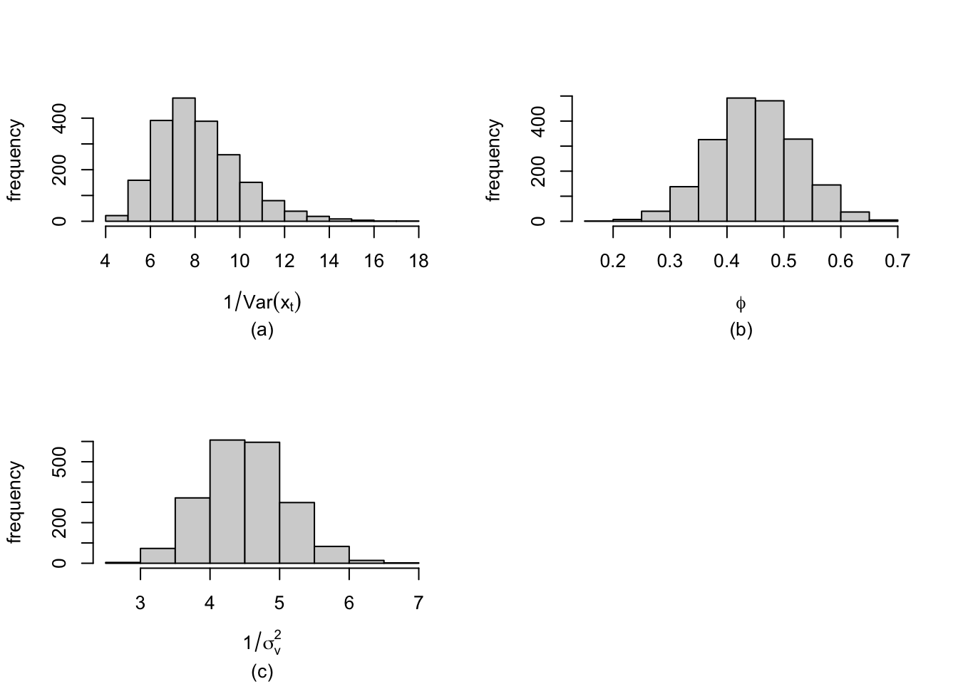
FIGURE 3.15: Histograms of samples of hyperparameters generated using the function inla.hyperpar.samples in the AR(1) with level plus noise model. Precision of state variable in (a), \(\phi\) in (b), and precision of the observation error in (c).

Next, we generate posterior samples for the latent random effects \(x_t, t=1,\ldots,n\). We set num.threads=1, and a random seed to facilitate reproducibility (see below for a discussion).

ar1.level.latent_hyper.samples <-
  inla.posterior.sample(n.samp,
                        model.ar1.level,
                        seed = 123457,
                        num.threads = 1)
length(ar1.level.latent_hyper.samples)
## [1] 2000
model.ar1.level$misc$configs$contents
## $tag
## [1] "Predictor"   "id.x"        "(Intercept)"
## 
## $start
## [1]    1  501 1001
## 
## $length
## [1] 500 500   1
names(ar1.level.latent_hyper.samples[[1]])
## [1] "hyperpar" "latent"   "logdens"

It is possible to look at time series plots of selected posterior \(x_t\) samples; for example, samples 500, 1000, 1500, and 2000 are shown in Figure 3.16.

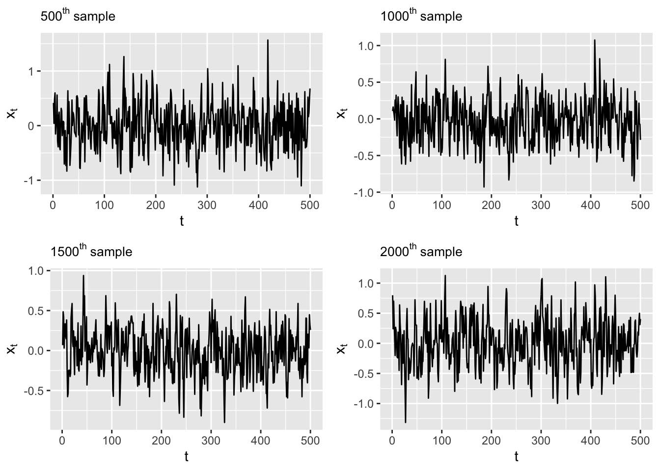
FIGURE 3.16: Time series plots of selected posterior samples from the AR(1) with level plus noise model.

Based on samples of size n.samp = 2000 we can construct histograms at selected times, say at \(t=250\) and time \(t=500\), as shown in Figure 3.17.

latent.sample.time <- ar1.level.latent_hyper.samples %>%
  sapply(function(x)
    x$latent[501:1000])
par(mfrow = c(1, 2))
hist(latent.sample.time[, 250],
     xlab = expression(x[250]),
     ylab = "frequency",
     main = "")
hist(latent.sample.time[, 500],
     xlab = expression(x[500]),
     ylab = "frequency",
     main = "")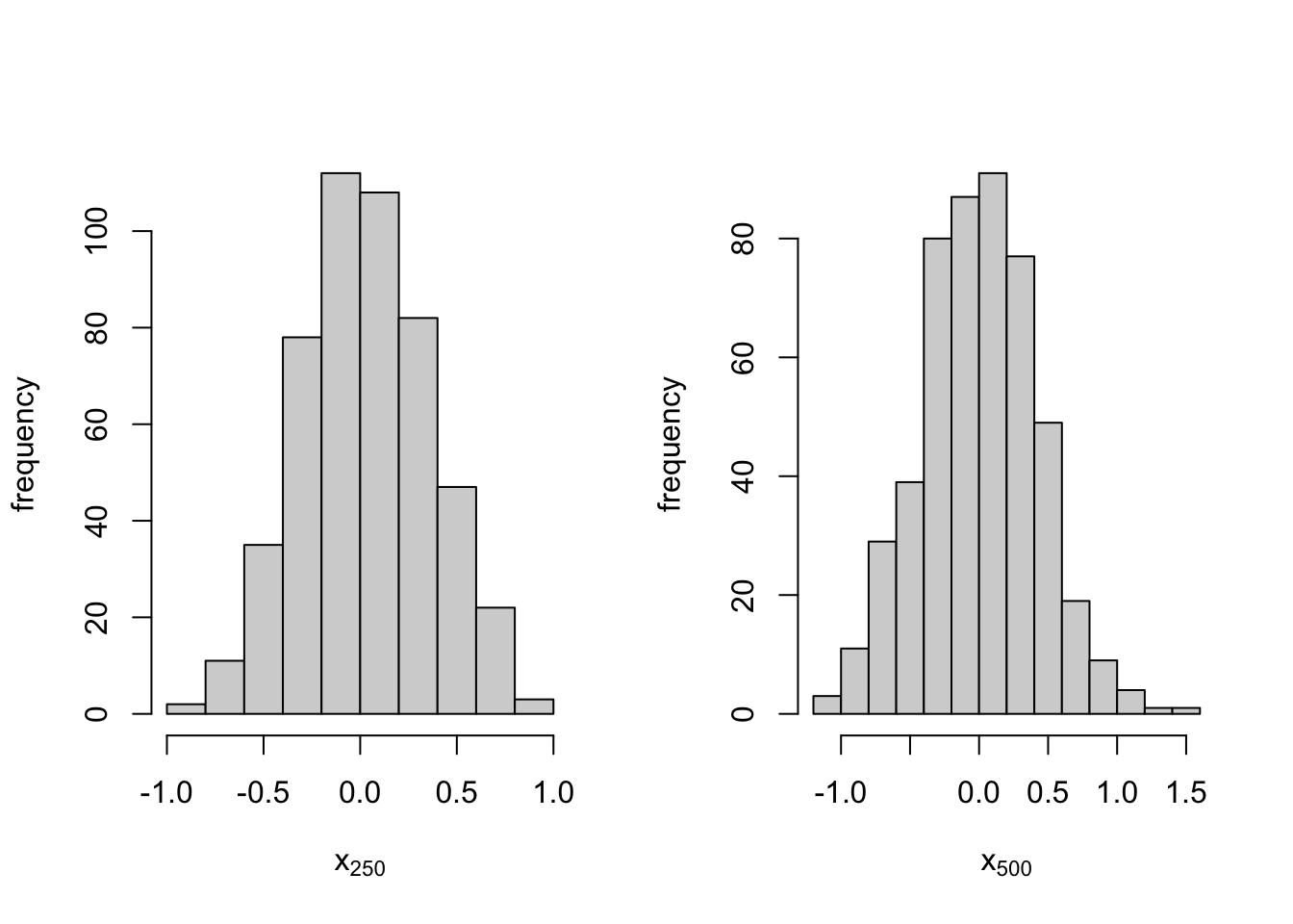

FIGURE 3.17: Histograms of posterior samples of the latent state for specific time points, t = 250 and t = 500, from the AR(1) model with level plus noise model.

We can obtain the predictive value \(\hat{y}_t = E(y_t|y_1,\ldots,y_n)\) as follows:

ar1.level.latent_hyper.samples[[1]]$latent[1:n]

These can also be computed manually using posterior samples of \(x_t\) and \(\alpha\):

ar1.level.latent_hyper.samples[[1]]$latent[(n + 1):(2 * n)]
+ tail(ar1.level.latent_hyper.samples[[1]]$latent, 1)

While the values of \(\hat{y}_t\) obtained from the two methods above are close, they do not coincide, as pointed out in Rue, Martino, and Chopin (2009).

A note on reproducibility

R-INLA uses the OpenMP multiple processing interface. It uses multiple cores on shared memory by default; i.e., it uses all cores available in a machine for computation. Due to machine differences, small variations can be observed while running the same code on different machines and perhaps when repeating runs on any machine, depending on available cores. One can specify the number of cores by using the option num.threads in inla(), higher values offering speedup. Setting num.threads = 1 can ensure exact reproducibility. See X. Wang, Yue, and Faraway (2018) and R-INLA discussion group.⁴

3.11 Posterior predictive samples of unknown observations

In many time series examples, it is very useful to use the posterior samples of the latent effects and hyperparameters in order to generate samples from the posterior predictive distributions of unknown observations (responses) given the observed data. The function inla.posterior.sample.eval() can be used to do this, as shown in the following code.

The function inla.posterior.sample.eval calls the function fun.pred() in order to compute the posterior predictive samples of the holdout data (last \(n_h = 5\) observations denoted as NA in the data frame).

fun.pred <- function(idx.pred) {
  m <- length(idx.pred)
  return (Predictor[idx.pred] + rnorm(m, mean = 0,
                                      sd = sqrt(1 / theta[1])))
}
pred.post <-
  inla.posterior.sample.eval(fun.pred, ar1.level.latent_hyper.samples,
                             idx.pred = which(is.na(y.append)))

In Figure 3.18, we show plots of time series of the 500-th, 1000-th, 1500-th, and 2000-th posterior predictive samples for the holdout period, together with all the observed values of the time series.

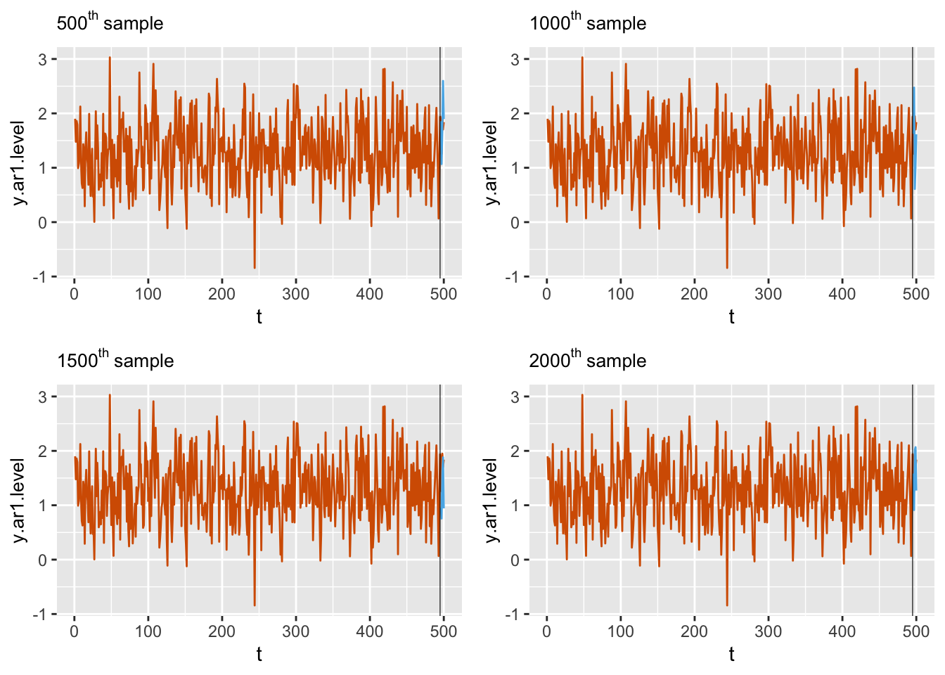
FIGURE 3.18: Comparing predictions (blue) of \(n_h=5\) holdout data and observed data (red). The black vertical line splits the data into the training and test sets.

We can also look at the histograms of the posterior predictive samples at times \(t=496\) and \(t=500\); see Figure 3.19.

par(mfrow = c(1, 2))
hist(pred.post[1, ],
     xlab = expression(x[496]),
     ylab = "frequency",
     main = "")
hist(pred.post[5, ],
     xlab = expression(x[500]),
     ylab = "frequency",
     main = "")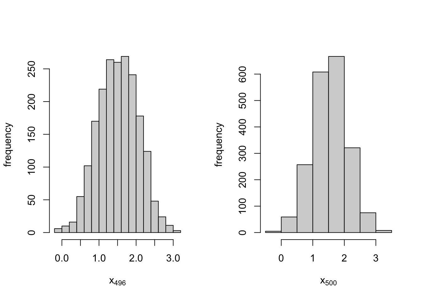

FIGURE 3.19: Histograms of posterior predictive samples for holdout time points t = 496 and t = 500 for the AR(1) with level plus noise model.

A comparison of the posterior means of the \(n_h = 5\) holdout points obtained from summary.fitted.values and from the posterior predictive samples shows that they are very similar.

dim(pred.post)
## [1]    5 2000
tail(model.ar1.level$summary.fitted.values$mean, 5)
## [1] 1.526 1.409 1.583 1.549 1.547
unname(rowMeans(pred.post))
## [1] 1.515 1.424 1.591 1.579 1.546

We end this chapter with Table 3.1 that gives a quick reference for the correspondence between terms in R-INLA summaries in their output and the terms in the DLMs. As mentioned earlier, note that Rho for id.x denotes \(\phi\) in the AR(1) model.

TABLE 3.1: Description of variables from inla() output.

Variable in INLA output	Math Notation	Description
Precision for the Gaussian observations	\(1/\sigma^2_v\)	Observation noise precision
Precision for id.w	\(1/\sigma^2_w\)	State noise precision
Precision for id.x	\(1/\sigma^2_x\)	State variable precision
Rho for id.x	\(\phi\)	AR(1) coefficient
id.delta	\(\delta\)	Drift in the state equation
(Intercept)	\(\alpha\)	Level in the observation equation

Chapter 3 – Appendix

Sampling properties of time series

Let \(X_{t}\) be a stationary time series.

1. Sample autocovariance function (ACVF)

The sample autocovariance function (ACVF) of \(X_{t}\) at lag \(h\) is

\[\begin{align} \widehat{\gamma}(h) = \dfrac{1}{n} \sum_{t=1}^{n-|h|} (x_{t+|h|}-\overline{x})(x_{t}-\overline{x}), \hspace{0.1in} -n < h < n. \tag{3.30} \end{align}\] Then, \(\widehat{\gamma}(0)\) is the sample variance of the time series.

2. Sample autocorrelation function (ACF)

The sample autocorrelation function (ACF) of \(X_{t}\) at lag \(h\) is

\[\begin{align} \widehat{\rho}(h) = \widehat{\gamma}(h) / \widehat{\gamma}(0), \hspace{0.1in} -n < h<n; \tag{3.31} \end{align}\] \(\widehat{\rho}(0)=1\) and \(|\widehat{\rho}(h)| \le 1,~ h=\pm 1, \pm2,\ldots\).

3. Sample spectrum-smoothed periodogram

Let \(i =\sqrt{-1}\), and let \(\omega_{j} = j/n\), for \(j=0,\ldots,n-1\) denote the Fourier frequencies. Define the complex-valued discrete Fourier transform (DFT) of \(X_{t}\) as

\[\begin{align} d(\omega_{j}) = \dfrac{1}{\sqrt{n}} \sum_{t=1}^{n} X_{t} \exp(-2 \pi i \omega_{j} t). \tag{3.32} \end{align}\] The periodogram of \(X_t\) is the (real-valued) estimate of its spectral density function and is defined as

\[\begin{align} I(\omega_{j}) = |d(\omega_{j})|^{2}. \tag{3.33} \end{align}\] The smoothed periodogram is a consistent estimate of the true spectrum of \(X_t\) and is obtained by averaging the periodogram ordinates over a frequency band of \(L < < n\) contiguous Fourier frequencies centered around \(\omega_{j}\). For example, the smoothed spectrum with the Daniell window is defined by

\[\begin{align} \hat{f}(\omega_{j}) = \dfrac{1}{L} \sum_{k=-m}^{m} I(\omega_{j} + \dfrac{k}{n}), \tag{3.34} \end{align}\] where, \(L = 2m+1\). The modified Daniell kernel is such that the two endpoints in the averaging get half the weight that the interior points get.

Autoregressive models

The AR\((p)\) model is widely used in time series modeling and forecasting. Here, \(p\) is an integer which denotes the order of the model. The mean form of the AR\((p)\) model is defined as

\[\begin{align} x_t -\mu = \phi_1 (x_{t-1} -\mu)+\phi_2 (x_{t-2} -\mu)+\ldots+\phi_p (x_{t-p} -\mu) + w_t, \tag{3.35} \end{align}\] while its intercept form is

\[\begin{align} x_t = \delta + \phi_1 x_{t-1} +\phi_2 x_{t-2} +\ldots+\phi_p x_{t-p} + w_t, \tag{3.36} \end{align}\] where \(\delta = (1-\phi_1 -\phi_2 -\ldots -\phi_p)\mu\). Using the backshift operator \(B\), with \(B^r x_t = x_{t-r}\), we can write the mean form and intercept form of the AR\((p)\) model in operator notation as

\[\begin{align} (1-\phi_1 B -\ldots -\phi_p B^p)(x_t -\mu) &= w_t, \mbox{ or }\tag{3.37}\\ (1-\phi_1 B -\ldots -\phi_p B^p)x_t &= \delta + w_t. \tag{3.38} \end{align}\] The AR\((p)\) process is stationary if the modulus of the roots of the AR polynomial equation

\[\begin{align} \phi(z) = 1-\phi_{1} z -\ldots - \phi_{p} z^{p} = 0 \tag{3.39} \end{align}\] are all greater than \(1\). Recall that a polynomial equation of order \(p\) will have \(p\) roots. These roots may all be real, or some roots may be real, while other roots are conjugate complex. The modulus of a real root is its absolute value, while the modulus of a complex root \(a+ib\) or \(a-ib\) is \(\sqrt{a^2+b^2}\). We can use the R function polyroot() to find the roots of the AR polynomial equation, and verify whether the modulus of each root is greater than \(1\). In the polyroot() function, an \(\ell^{th}\) order polynomial must be written in the form \(p(z) = c_1 + c_2 z +\ldots+ c_{\ell+1} z^\ell\), where the \(c_j,~j=1,\ldots,\ell+1\) are constants. For example, consider the AR\((2)\) process

\[\begin{align*} (1-\phi_{1}B - \phi_{2} B^{2})x_t= w_t, \end{align*}\] with \(\phi_1=1.5\) and \(\phi_2=-0.75\). The AR\((2)\) polynomial is \(p(z) =(1-1.5 z+0.75z^2)\), and
the equation \(p(z)=0\) has two conjugate complex roots, i.e., \(z[1]=1+0.57735i\) and \(z[2]=1-0.57735 i\), where \(i =\sqrt{-1}\). The modulus of these roots is \(1.1547 >1\); hence this AR\((2)\) process is stationary.

phi1 <- 1.5
phi2 <- -0.75
u <- polyroot(c(1,-phi1,-phi2))
u[1]
## [1] 1+0.577i
u[2]
## [1] 1-0.577i
Mod(u[1])
## [1] 1.155
Mod(u[2]) 
## [1] 1.155

The stationarity region for an AR\((p)\) process is a convex set \(C_p \subset \mathbb{R}^p\), and involves nonlinear constraints on \(\boldsymbol{\phi}=(\phi_1^p,\ldots, \phi_p^p)'\) To handle this, R-INLA uses the partial autocorrelation function (PACF) parameterization from \(C_p\) to the \(p\)-dimensional hypercube \((-1,1)^p\) (see Barndorff-Nielsen and Schou (1973) and Marriott et al. (1996)). The one-to-one transformation with partial autocorrelations \(\boldsymbol r = (r_1, \ldots, r_p)'\) is

\[\begin{align*} \phi_{k}^{(k)} &= r_k \notag \\ \phi_{i}^{(k)} &= \phi_{i}^{(k-1)} -r_k \phi_{k-i}^{(k-1)},~i=1,\ldots, k-1. \end{align*}\] Monahan (1984) gave the inverse transformation as

\[\begin{align} \phi_{i}^{(k-1)}=\frac{\phi_{i}^{(k)} +\phi_{k}^{(k)}\phi_{k-i}^{(k)}} {(1-\phi_{k}^{(k)})^2},~i=1,\ldots,k-1, \tag{3.40} \end{align}\] with Jacobian

\[\begin{align} J = \prod_{k=1}^p (1-r_k^2)^{\frac{(k-1)}{2}} \prod_{j=1}^{[p/2]}(1-r_{2j}). \tag{3.41} \end{align}\] In R-INLA, the partial autocorrelations of an AR\((p)\) model are denoted by \(\psi_k\), with \(|\psi_k| <1\) for \(k=1,\ldots,p\). In terms of the internal parameterization, for \(k=1,\ldots,p\),

\[\begin{align*} \psi_k = 2 \frac{\exp(\theta_{\psi,k})}{1+\exp(\theta_{\psi,k})} -1. \end{align*}\] For an AR(2) process, these transformations are obtained as follows.

# phi to pacf
phi <- c(phi1, phi2)
pacf <- inla.ar.phi2pacf(phi)
#pacf to phi
phi.1 <- inla.ar.pacf2phi(pacf)

References

Barndorff-Nielsen, Ole E., and Geert Schou. 1973. “On the Parameterization of Autoregressive Models by Partial Autocorrelations.” Journal of Multivariate Analysis 3 (4): 408–19.

Boehmke, Bradley C. 2016. Data Wrangling with r. Switzerland: Springer International Publishing.

Fuglstad, Geir-Arne, Daniel Simpson, Finn Lindgren, and Håvard Rue. 2019. “Constructing Priors That Penalize the Complexity of Gaussian Random Fields.” Journal of the American Statistical Association 114 (525): 445–52.

Gamerman, D., and F. H. Lopes. 2006. Markov Chain Monte Carlo: Stochastic Simulation for Bayesian Inference. New York: Chapman & Hall/CRC.

Gómez-Rubio, Virgilio. 2020. Bayesian Inference with INLA. Boca Raton, Florida: CRC Press.

Gómez-Rubio, Virgilio, and Håvard Rue. 2018. “Markov Chain Monte Carlo with the Integrated Nested Laplace Approximation.” Statistics and Computing 28 (5): 1033–51.

Kalman, Rudolph Emil. 1960. “A New Approach to Linear Filtering and Prediction Problems.” Trans. ASME J. Basic Engineering 83.

Marriott, John, Nalini Ravishanker, Alan E. Gelfand, and Jeffrey S. Pai. 1996. “Bayesian Analysis of ARMA Processes: Complete Sampling-Based Inference Under Exact Likelihoods.” Bayesian Analysis in Statistics and Econometrics, 243–56.

Monahan, John F. 1984. “A Note on Enforcing Stationarity in Autoregressive-Moving Average Models.” Biometrika 71 (2): 403–4.

Rue, Håvard, and Leonhard Held. 2005. Gaussian Markov Random Fields: Theory and Applications. Boca Raton, Florida: Chapman & Hall/CRC.

Rue, Håvard, Sara Martino, and Nicholas Chopin. 2009. “Approximate Bayesian Inference for Latent Gaussian Models Using Integrated Nested Laplace Approximations (with Discussion).” Journal of the Royal Statistical Society, Series B 71: 319–92.

Ruiz-Cárdenas, Ramiro, Elias T. Krainski, and Håvard Rue. 2012. “Direct Fitting of Dynamic Models Using Integrated Nested Laplace Approximations—INLA.” Computational Statistics & Data Analysis 56 (6): 1808–28.

Seppä, Karri, Håvard Rue, Timo Hakulinen, Esa Läärä, Mikko J. Sillanpää, and Janne Pitkäniemi. 2019. “Estimating Multilevel Regional Variation in Excess Mortality of Cancer Patients Using Integrated Nested Laplace Approximation.” Statistics in Medicine 38 (5): 778–91.

Shumway, Robert H., and David S. Stoffer. 2017. Time Series Analysis and Its Applications: With r Examples. Springer Texts in Statistics. New York: Springer International Publishing.

Wang, Xiaofeng, Yuryan Yue, and Julian J. Faraway. 2018. Bayesian Regression Modeling with INLA. New York: Chapman; Hall/CRC.

Wickham, Hadley. 2016. Ggplot2: Elegant Graphics for Data Analysis. New York: Springer-Verlag. https://ggplot2.tidyverse.org.

Wickham, Hadley, Mara Averick, Jennifer Bryan, Winston Chang, Lucy D’Agostino McGowan, Romain François, Garrett Grolemund, et al. 2019. “Welcome to the tidyverse.” Journal of Open Source Software 4 (43): 1686. https://doi.org/10.21105/joss.01686.