Chapter 6 Hierarchical Dynamic Models for Panel Time Series
6.1 Introduction
Multilevel or hierarchical models are widely used and have also been implemented in R (Gelman and Hill 2006). In Chapter 4 of their book, Gómez-Rubio (2020) discuss R-INLA implementation for hierarchical models, including longitudinal data models; also see Krainski et al. (2018). In this chapter, we describe approximate dynamic Bayesian analysis
for a set of \(g\) univariate time series. Such time series are also referred to as panel time series in the literature. Balaji Raman et al. (2021) describe an interesting application in the marketing domain. An alternate hierarchical Bayesian DLM framework for Gaussian time series has been discussed in D. Gamerman and Migon (1993).
In Section 6.2, we use simulated data to show how to fit models to \(g\) time series when we assume that the parameters in the AR(1) state evolution equation are assumed to be the same. Parameters such as the level \(\alpha\) in the observation equation can exhibit considerable variation, and may be modeled as a fixed or random effect. Section 6.3 shows a few plausible hierarchical models for NYC ridesourcing usage data.
The custom functions must first be sourced by the user.
source("functions_custom.R")We use the following packages.
library(tables)
library(tidyverse)
library(INLA)
We analyze the following data.
- Ridesourcing in NYC
6.2 Models with homogenous state evolution
Consider \(g\) time series each of length \(n\). Let \(Y_{it}\) denote the continuous-valued response at time \(t\) for the \(i\)th series, \(i=1,\ldots,g\) and \(t=1,\ldots,n\). The response can be written as a data matrix \(\boldsymbol Y\) with \(g\) rows (subjects/locations) and \(n\) columns (time points):
\[\begin{align} \boldsymbol Y = \begin{pmatrix} y_{11} & y_{12} & \ldots & y_{1n} \\ y_{21} & y_{22} & \ldots & y_{2n} \\ \vdots & \vdots & \ddots & \vdots \\ y_{g1} & y_{g2} & \ldots & y_{gn} \end{pmatrix}. \tag{6.1} \end{align}\] In all the models below, \(v_{it}\) and \(w_{it}\) are uncorrelated, with \(v_{it}\) being i.i.d. N\((0,\sigma^2_v)\) and \(w_{it}\) being i.i.d. N\((0,\sigma^2_w)\)
6.2.1 Example: Simulated homogeneous panel time series with the same level
Consider the following model for \(y_{it}\):
\[\begin{align} y_{it} &= \alpha + \beta_{it,1} Z_{it} + v_{it}, \notag \\ \beta_{it,1} &= \phi \beta_{i,t-1,1}+ w_{it}, \tag{6.2} \end{align}\] where the coefficient \(\beta_{it,1}\) corresponding to the exogenous predictor \(Z_{it}\) evolves over time as an AR(1) process for each \(i\). The \(g\) series have very similar stochastic behavior as indicated by having (nearly) the same values of \(\phi\), \(\sigma^2_v\), and \(\sigma^2_w\). The level of each series is assumed to be the same value \(\alpha\).
set.seed(123457)
g <- 100
n <- 250
burn.in <- 500
n.tot <- n + burn.in
alpha <- 10.0
sigma2.w0 <- 0.25
sigma2.v0 <- 1.0
phi.0 <- 0.8
The code below generates the response and predictors.
yit.all <-
  yit.all.list <-
  z1.all <- z2.all <- z.all <- sigma2.w <- vector("list", g)
for (j in 1:g) {
  yit <- beta.1t  <- z <- vector("double", n.tot)
  u <- runif(1, min = -0.1, max = 0.05)
  phi <- phi.0 + u
  us <- runif(1, min = -0.15, max = 0.25)
  sigma2.w[[j]] <- sigma2.w0 + us
  beta.1t <-
    arima.sim(list(ar = phi, ma = 0), n = n.tot, sd = sqrt(sigma2.w[[j]]))
  z <- rnorm(n.tot)
  v <- rnorm(n.tot)
  for (i in 1:n.tot) {
    yit[i] <- alpha + beta.1t[i]  * z[i] + v[i]
  }
  yit.all.list[[j]] <- tail(yit, n)
  z.all[[j]] <- tail(z, n)
}
yit.all <- unlist(yit.all.list)
z.all <- unlist(z.all)
We set up indexes, replicates, data frame, and the formula.
id.beta1 <- rep(1:n, g)
re.beta1  <- rep(1:g, each = n)
data.panelts.1 <-
  cbind.data.frame(id.beta1, z.all, yit.all, re.beta1)
formula.panelts.1 <-
  yit.all ~ 1  +
  f(id.beta1, z.all, model = "ar1", replicate = re.beta1)
We fit the model and summarize the results.
model.panelts.1 <- inla(
  formula.panelts.1,
  family = "gaussian",
  data = data.panelts.1,
  control.predictor = list(compute = TRUE, link = 1),
  control.compute = list(
    dic = TRUE,
    cpo = TRUE,
    waic = TRUE,
    config = TRUE,
    cpo = TRUE
  )
)format.inla.out(model.panelts.1$summary.fixed)
## name mean sd 0.025q 0.5q 0.975q mode kld
## 1 Intercept 9.999 0.007 9.985 9.999 10.01 9.999 0
format.inla.out(model.panelts.1$summary.hyperpar[,c(1:2)])
## name mean sd
## 1 Precision for Gaussian obs 1.009 0.012
## 2 Precision for id.beta1 1.302 0.036
## 3 Rho for id.beta1 0.778 0.009The results for the fixed and random parameters show that all the parameters are adequately recovered.
6.2.2 Example: Simulated homogeneous panel time series with different levels
Consider the following model:
\[\begin{align} y_{it} &= \alpha_i + \beta_{it,1} Z_{it} + v_{it}, \notag \\ \beta_{it,1} &= \phi \beta_{i,t-1,1}+ w_{it}, \tag{6.3} \end{align}\] where the coefficient \(\beta_{it,1}\) corresponding to the exogenous predictor \(Z_{it}\) evolves over time as an AR(1) process for each \(i\). The \(g\) series have very similar stochastic behavior as indicated by having (nearly) the same values of \(\phi\), \(\sigma^2_v\), and \(\sigma^2_w\). The levels \(\alpha_i\) are assumed to be possibly different across the \(g\) series. If \(g\) is small, the \(\alpha_i\) coefficients may be treated as fixed effects. On the other hand, when \(g\) is large, it is usual to assume that \(\alpha_i\) are random effects assumed to follow a N\((0,\sigma^2_\alpha)\) distribution, with unknown \(\sigma^2_\alpha\).
Case 1
Assume that \(g=10\), and \(\alpha_i\) are fixed effects. We employ the
fact.alpha <- as.factor(id.alpha) to set up the \(g\) levels to include in the formula. The true parameters
sigma2.w0, sigma2.v0, phi.0, n, and burn.in are the same as in the previous example. The response and predictors are generated as follows.
yit.all <-
  yit.all.list <-
  z1.all <- z2.all <- alpha <- z.all <- sigma2.w <- vector("list", g)
for (j in 1:g) {
  yit <- beta.1t  <- z <- vector("double", n.tot)
  u <- runif(1, min = -0.1, max = 0.05)
  phi <- phi.0 + u
  us <- runif(1, min = -0.15, max = 0.25)
  sigma2.w[[j]] <- sigma2.w0 + us
  beta.1t <-
    arima.sim(list(ar = phi, ma = 0), n = n.tot, sd = sqrt(sigma2.w[[j]]))
  alpha[[j]] <- sample(seq(-2, 2, by = 0.1), 1)
  z <- rnorm(n.tot)
  v <- rnorm(n.tot)
  for (i in 1:n.tot) {
    yit[i] <- alpha[[j]] + beta.1t[i]  * z[i] + v[i]
  }
  yit.all.list[[j]] <- tail(yit, n)
  z.all[[j]] <- tail(z, n)
}
yit.all <- unlist(yit.all.list)
z.all <- unlist(z.all)
The indexes, replicates, data frame, and the formula follow.
id.beta1 <- rep(1:n, g)
re.beta1 <- id.alpha <- rep(1:g, each = n)
fact.alpha <- as.factor(id.alpha)
data.panelts.2 <-
  cbind.data.frame(id.beta1, z.all, yit.all, re.beta1, fact.alpha)
formula.panelts.2 <-
  yit.all ~ -1 + fact.alpha +
  f(id.beta1, z.all, model = "ar1", replicate = re.beta1)
We save the output from the fit in model.panelts.2 using code similar to that in the previous example, but using formula.panelts.2 and data.panelts.2 as inputs.
model.panelts.2 <- inla(
  formula.panelts.2,
  family = "gaussian",
  data = data.panelts.2,
  control.predictor = list(compute = TRUE, link = 1),
  control.compute = list(
    dic = TRUE,
    cpo = TRUE,
    waic = TRUE,
    config = TRUE,
    cpo = TRUE
  )
)format.inla.out(summary.model.panelts.2$fixed[,c(1,2,4)])
## name mean sd 0.5q
## 1 fact.alpha1 0.470 0.070 0.470
## 2 fact.alpha2 -0.511 0.072 -0.511
## 3 fact.alpha3 0.162 0.071 0.162
## 4 fact.alpha4 0.728 0.069 0.728
## 5 fact.alpha5 1.395 0.070 1.395
## 6 fact.alpha6 -1.311 0.070 -1.311
## 7 fact.alpha7 -0.551 0.072 -0.551
## 8 fact.alpha8 0.998 0.070 0.998
## 9 fact.alpha9 -1.064 0.070 -1.064
## 10 fact.alpha10 -0.352 0.072 -0.352
format.inla.out(summary.model.panelts.2$hyperpar[,c(1:2)])
## name mean sd
## 1 Precision for Gaussian obs 1.065 0.042
## 2 Precision for id.beta1 1.230 0.103
## 3 Rho for id.beta1 0.760 0.026The posterior means of \(\alpha_i\) are close to the true values given by
unlist(alpha)
##  [1]  0.4 -0.5  0.2  0.8  1.5 -1.4 -0.6  0.9 -1.1 -0.4
Case 2
We next show the code for treating \(\alpha_i\)’s as independent N\((0,\sigma^2_\alpha)\) random variables, instead of treating them as fixed coefficients. This is useful when \(g\) is large; here \(g=100\).
In this case, we model the random levels via f(id.alpha, model="iid"), as shown below. The true parameters
sigma2.w0, sigma2.v0, phi.0, n, and burn.in are the same as in the previous example. The response and predictors are generated as follows.
yit.all <-
  yit.all.list <-
  z1.all <- z2.all <- alpha <- z.all <- sigma2.w <- vector("list", g)
for (j in 1:g) {
  yit <- beta.1t  <- z <- vector("double", n.tot)
  u <- runif(1, min = -0.1, max = 0.05)
  phi <- phi.0 + u
  us <- runif(1, min = -0.15, max = 0.25)
  sigma2.w[[j]] <- sigma2.w0 + us
  beta.1t <-
    arima.sim(list(ar = phi, ma = 0), n = n.tot, sd = sqrt(sigma2.w[[j]]))
  alpha[[j]] <- sample(seq(-2, 2, by = 0.1), 1)
  z <- rnorm(n.tot)
  v <- rnorm(n.tot)
  for (i in 1:n.tot) {
    yit[i] <- alpha[[j]] + beta.1t[i]  * z[i] + v[i]
  }
  yit.all.list[[j]] <- tail(yit, n)
  z.all[[j]] <- tail(z, n)
}
yit.all <- unlist(yit.all.list)
z.all <- unlist(z.all)
The indexes, replicates, data frame, and formula follow.
id.beta1 <- rep(1:n, g)
re.beta1 <- id.alpha <- rep(1:g, each = n)
data.panelts.3 <-
  cbind.data.frame(id.beta1, z.all, yit.all, re.beta1, id.alpha)
formula.panelts.3 <-
  yit.all ~ -1 + f(id.alpha, model="iid") +
  f(id.beta1, z.all, model = "ar1", replicate = re.beta1)
We save the output from the fit in model.panelts.3 using code similar to that in the previous example, but using formula.panelts.3 and data.panelts.3 as inputs.
model.panelts.3 <- inla(
  formula.panelts.3,
  family = "gaussian",
  data = data.panelts.3,
  control.predictor = list(compute = TRUE, link = 1),
  control.compute = list(
    dic = TRUE,
    cpo = TRUE,
    waic = TRUE,
    config = TRUE,
    cpo = TRUE
  )
)format.inla.out(model.panelts.3$summary.hyperpar[,c(1:2)])
## name mean sd
## 1 Precision for Gaussian obs 1.006 0.013
## 2 Precision for id.alpha 0.577 0.075
## 3 Precision for id.beta1 1.349 0.051
## 4 Rho for id.beta1 0.789 0.008Note that in this case, as in the case of treating the levels as fixed effects, we recover the true \(\phi\), \(\sigma_v^2\) and \(\sigma_w^2\). For random \(\alpha_i\), we notice that the estimated posterior precision matches the true precision of the simulated random \(\alpha\)’s shown below. The overall estimation accuracy should increase as \(g\) increases.
1/var(unlist(alpha))
## [1] 0.8016
In practice, we may often need to model multiple time series for which the stochastic behavior may differ between series. For instance, in (6.3), we may wish to model the state equation as
\[\begin{align} \beta_{it,1} = \phi_i \beta_{i,t-1,1}+ w_{it}, \tag{6.4} \end{align}\] where \(w_{it}\) are N\((0,\sigma^2_{w_i})\) variables. We discuss such models after describing an approach for multivariate time series in Chapter 12.
Remark: More on the replicate argument.
Recall that we used the copy option in Chapter 5. If a model includes several likelihood terms, it may be necessary to share some terms among different parts of the model.
In R-INLA, we can use the replicate feature to enable the linear predictors of the different likelihoods to share the same type of latent effect.
Unlike the copy feature, replicate allows different hyperparameters for each replicate of an effect.
The hyperparameter estimation will be based on all the data, but estimates of the latent effects are allowed to vary between the groups.
6.3 Example: Ridesourcing in NYC
Transportation Network Companies (TNCs) provide ridesourcing services by allowing passengers to use their smart phone apps to connect with nearby drivers who typically drive part-time using their own car. We consider weekly ridesourcing usage data from \(g=105\) different taxi zones in NYC from January 2015 until June 2017, providing data for \(n=129\) weeks. The data consists of TNC, Taxi, and Subway usage by taxi zones for each week. TNC usage aggregates three ride modes: Uber, Lyft, and Via. Taxi usage aggregates Yellow and Green Cabs. In most of the zones, TNC usage shows a continuous increase over time, while Taxi usage exhibits a decreasing trend. Subway usage, as expected for NYC, dominates the other two in most zones. The data set also includes data on potential predictors, obtained from various sources such as the NYC Open Data Portal, National Oceanic and Atmospheric Administration (NOAA), the U.S. Census Bureau, etc.; see Gerte et al. (2019) and Toman et al. (2020) for details. They include: (a) data that varies by week but remains constant across all taxi zones for any given week, such as holidays (an indicator) and precipitation (inches), and (b) data on socio-economic and land-use variables which we assume vary by taxi zones and consists of Total Population/No. of Buildings, Fulltime Employed/No. of Buildings, Median Age, and Median Earnings. Toman et al. (2020) described time series (ARIMA-GARCH) models to weekly ridesourcing usage within taxi zones in NYC, followed by an investigation into the existence of spatial dependence between the taxi zones. Since the stochastic patterns appear to be varying over time, use of hierarchical dynamic models is a natural choice for such data. Hierarchical models (Gelman and Hill 2006) enable us to pool information from \(g\) groups or individuals (taxi zones in our example) to estimate common coefficients as well as estimating group/zone-specific coefficients. Including time-varying effects in dynamic hierarchical models adds another level of complexity, as we show below.
In the dataset, we have divided each observed count by \(k=10,000\) and split the panel time series data into training (or calibration) and hold-out (or test) portions. Specifically, we set aside \(n_h=5\) weeks from each of the \(g=105\) taxi zones.
ride <-
  read.csv("tnc_weekly_data.csv",
           header = TRUE,
           stringsAsFactors = FALSE)
n <- n_distinct(ride$date)
g <- n_distinct(ride$zoneid)
k <- 10000
ride$tnc <- ride$tnc / k
ride$taxi <- ride$taxi / k
ride$subway <- ride$subway / k
# Train and test data
n.hold <- 5
n.train <- n - n.hold
df.zone <- ride %>%
  group_split(zoneid)
train.df <- df.zone %>%
  lapply(function(x)
    x[1:n.train,]) %>%
  bind_rows()
test.df <- df.zone %>%
  lapply(function(x)
    tail(x, n.hold)) %>%
  bind_rows()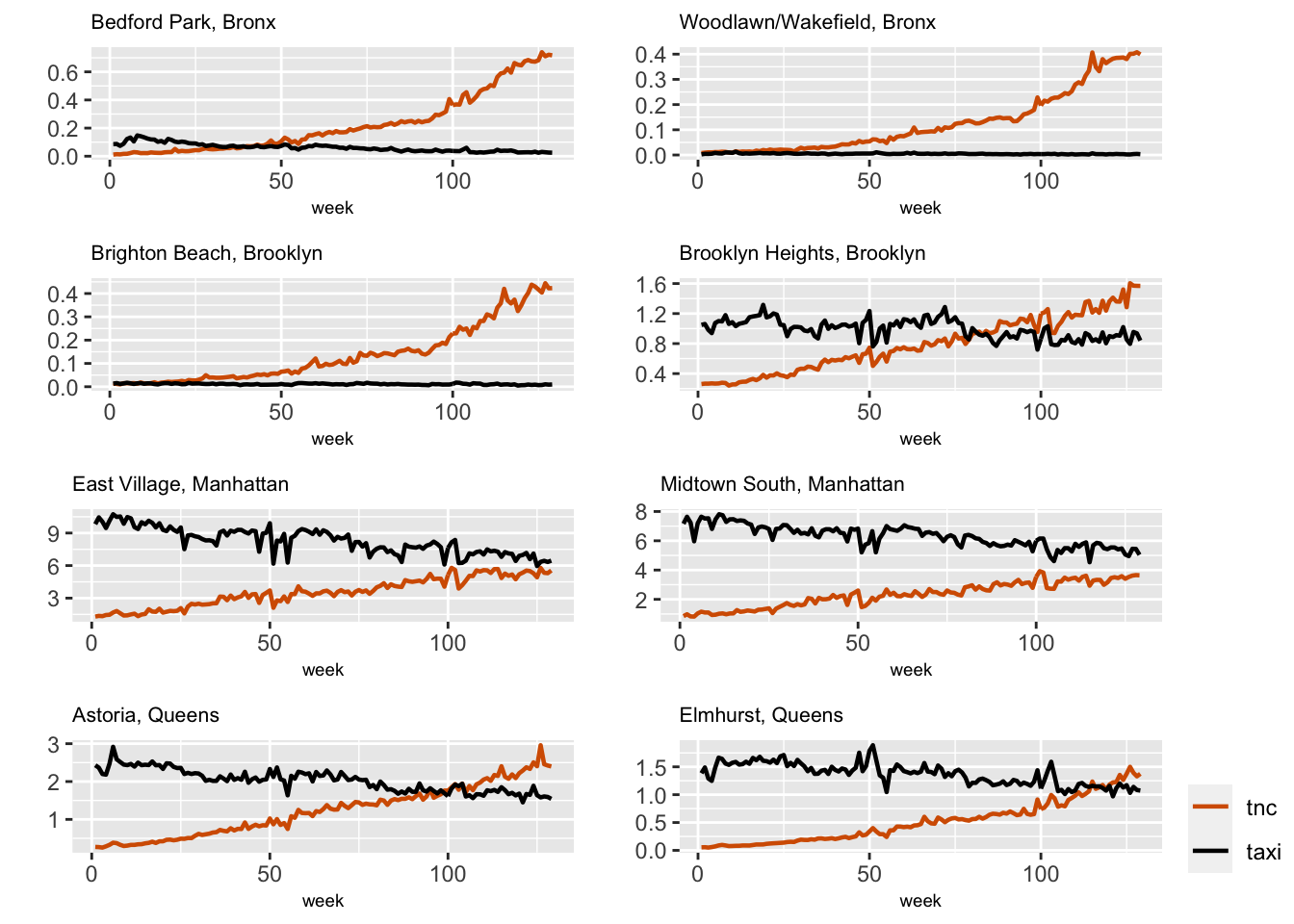
FIGURE 6.1: Scaled TNC and Taxi usage across eight taxi zones.
Figure 6.1 shows the scaled weekly usage of TNC and Taxi in two randomly selected taxi zones from four boroughs in NYC. We see that TNC usage shows an upward trend whereas Taxi usage exhibits an overall downward trend with some fluctuation. There are some similarities and differences in temporal patterns in the different zones, which we explore using hierarchical dynamic models. We first describe the variables used in these models.
Description of variables
The response time series \(Y_{it}\) are the scaled TNC usage in week \(t\) in zone \(i\), with \(n=129\) and \(g=105\). The response can be written as a data matrix \(\boldsymbol Y\) with \(g\) rows (subjects/locations) and \(n\) columns (time points); see (6.1). We consider three types of predictors:
Predictors that vary by week \(t\) and zone \(i\): these include Subway usage and Taxi usage, denoted by \(b_{it,1}\) and \(b_{it,2}\); let \(\boldsymbol{b}_{it} = (b_{it,1},b_{it,2})'\). In general, we can assume that there are \(c\) such predictors, indexed by \(h =1,\ldots,c\).
Predictors that only vary by week \(t\): these variables are constant across all taxi zones \(i\) for any given \(t\). They include holidays (an indicator) and precipitation (inches), which we denote by \(d_{t,1}\), and \(d_{t,2}\) respectively. Let \(\boldsymbol{d}_{t} = (d_{t,1},d_{t,2})'\). In general, we can assume that there are \(a\) such predictors, indexed by \(\ell =1,\ldots,a\).
Predictors that only vary by zone \(i\): these are assumed to stay constant week by week. They include scaled.population, scaled.employment, median.age, and median.earnings, and are denoted by \(s_{i,1}, s_{i,2}, s_{i,3}\), and \(s_{i,4}\) respectively; let \(\boldsymbol{s}_{i} = (s_{i,1}, s_{i,2}, s_{i,3},s_{i,4})'\). In general, we can assume that there are \(b\) such predictors.
Below, we describe and fit the most general hierarchical dynamic model for the ridesourcing data, i.e., Model H1.
6.3.1 Model H1. Dynamic intercept and exogenous predictors
Consider the following model for \(Y_{it}\):
\[\begin{align} Y_{it} &= \alpha + \beta_{it,0}+\boldsymbol{b}'_{it}\boldsymbol{\beta}_{it}+ \boldsymbol{d}'_{t}\boldsymbol{\gamma}_{t}+ \boldsymbol{s}'_{i}\boldsymbol{\eta}_{i}+ v_{it} \notag \\ \beta_{it,0} &= \phi_0 \beta_{i,t-1,0}+w_{it,0}, \notag \\ \beta_{it,h} &= \phi_h^{(\beta)} \beta_{i,t-1,h}+w^{(\beta)}_{it,h},~h=1,2, \notag \\ \gamma_{t,\ell} &= \phi_\ell^{(\gamma)} \gamma_{t-1,\ell}+w^{(\gamma)}_{t,\ell},~\ell=1,2. \label{tnc-stgamma} \end{align}\] We have included a level \(\alpha\), and a time-varying intercept \(\beta_{it,0}\) which is modeled as a latent zero-mean AR(1) process with coefficient \(\phi_0\). The coefficients corresponding to Subway usage and Taxi usage are \(\beta_{it,h},~h=1,2\), each of which evolves as a latent Gaussian AR(1) process with coefficients \(\phi_1^{(\beta)}\) and \(\phi_2^{(\beta)}\) respectively. The coefficients corresponding to holidays and precipitation are \(\gamma_{t,\ell},~\ell=1,2\), and evolve as latent Gaussian AR(1) processes with coefficients \(\phi_1^{(\gamma)}\) and \(\phi_2^{(\gamma)}\) respectively. The \(\boldsymbol{\eta}_{i}\) coefficients corresponding to the demographic and land-use predictors are only taxi-zone specific and do not follow any dynamic model. We assume that all the AR(1) coefficients lie between \(-1\) and \(1\). The observation errors \(v_{it}\) are assumed to be N\((0, \sigma^2_v)\). The state errors \(w_{it,0}\) are N\((0,\sigma^2_{w,0})\), the errors \(w^{(\beta)}_{it,h}\) are N\((0,\sigma^2_{w,\beta_h}),~h=1,2\), and the errors \(w^{(\gamma)}_{t,\ell}\) are N\((0,\sigma^2_{w,\gamma_\ell}),~\ell=1,2\). The errors are uncorrelated. For elements of \(\boldsymbol{\eta}_{i}\) in the model, we assume independent normal priors. An important aspect of fitting Model H1 is the creation of indexes to handle the different types of coefficients described above (also see Chapter 6 of Gómez-Rubio (2020)).
Model H1: indexes and replicates
Indexes for time and zone varying coefficients. The time index id.b0 relates to the intercept \(\beta_{it,0}\) which varies by week \(t\) and zone \(i\). To capture the time-varying effect, we use
rep(1:n,g), which repeats the weeks \(1,\ldots,n\) for all \(g=105\) zones. To allow the intercept to vary by zones, we use thereplicateargument in the functionf(). Since the first set of times \(1,\ldots,n\) belongs to the first zone, \(i=1\), the index has \(1\) repeated \(n\) times; the next set of \(1,\ldots,n\) is for zone \(i=2\), so that the index is \(2\) repeated \(n\) times, and so on. This is represented byrep(1:g, each = n)for re.b0 in the formula. We similarly set up the indexes id.subway and id.taxi, as well as the replicates re.subway and re.taxi corresponding to \(\beta_{it,1}\) and \(\beta_{it,2}\) respectively.Indexes for time-varying coefficients. For the predictors holidays and precip, the \(\gamma\) coefficients vary only by time \(t\) and not by zone \(i\). The indexes id.holiday and id.precip are defined similar to id.b0, i.e., by
rep(1:n,g). However, thereplicateargument must be different. We define re.holiday as a column of \(1\)’s repeated \(n\times g\) times, i.e., byrep(1, (n*g)). In addition, we allow a large, fixed precision for the hyperparameter. The index and replicate arguments for precip are set up similarly.Indexes for zone specific coefficients. Since the \(\boldsymbol{\eta}_{i}\) coefficients corresponding to the demographic and land use predictors do not vary over time, but are zone specific, we do not need to set up indexes similar to id.b0. However, to indicate that they are random effects (by zone), we need to set up the replicate arguments re.age, re.earn, re.pop, and re.emp as repeating the sequence \(1,\ldots,g\) for each \(t\), i.e., by
,rep(1:g, each = n). These indexes and replicates for Model H1 are shown in the code below.
id.b0 <- id.subway <- id.taxi <- rep(1:n, g)
id.holiday <- id.precip <- rep(1:n, g)
re.b0 <- re.subway <- re.taxi <- rep(1:g, each = n)
re.holiday <- re.precip <- rep(1, (n * g))
re.age <- re.earn <- re.pop <- re.emp <- rep(1:g, each = n)
We merge these with the scaled data to create a data frame ride.data that is used in the inla() fit.
ride.data <-
  cbind.data.frame(
    ride,id.b0,id.subway,id.taxi,
    id.holiday,id.precip,re.b0,
    re.subway,re.taxi,re.holiday,
    re.precip,re.age,re.earn,re.pop,re.emp
  )
Model H1: formula and model fitting
formula.tnc.H1 <- tnc ~ 1 +
  f(id.b0, model = "ar1", replicate = re.b0) +
  f(id.subway, subway, model = "ar1", replicate = re.subway) +
  f(id.taxi, taxi, model = "ar1", replicate = re.taxi) +
  f(
    id.holiday,
    holidays,
    model = "ar1",
    replicate = re.holiday,
    hyper = list(theta = list(initial = 20, fixed = TRUE))
  ) +
  f(
    id.precip,
    precip,
    model = "ar1",
    replicate = re.precip,
    hyper = list(theta = list(initial = 20, fixed = TRUE))
  ) +
  f(re.age, median.age, model = "iid") +
  f(re.earn, median.earnings, model = "iid") +
  f(re.pop, scaled.population, model = "iid") +
  f(re.emp, scaled.employment, model = "iid")
We have used default R-INLA priors for all parameters. The condensed output shown below consists of posterior summaries from Model H1.
model.tnc.H1 <- inla(
  formula.tnc.H1,
  data = ride.data,
  control.predictor = list(compute = TRUE),
  control.compute = list(
    dic = TRUE,
    waic = TRUE,
    cpo = TRUE,
    config = TRUE
  )
)
format.inla.out(summary.model.tnc.H1$fixed)
format.inla.out(model.tnc.H1$summary.hyperpar[,c(1:2)])
## name mean sd 0.025q 0.5q 0.975q mode kld
## 1 Intercept -0.4 0.146 -0.686 -0.4 -0.114 -0.4 0## name mean sd
## 1 Precision for Gaussian obs 1.995e+03 7.805e+01
## 2 Precision for id.b0 2.156e+00 7.540e-01
## 3 Rho for id.b0 9.990e-01 0.000e+00
## 4 Precision for id.subway 6.815e+03 1.298e+03
## 5 Rho for id.subway 9.980e-01 0.000e+00
## 6 Precision for id.taxi 1.690e+00 3.520e-01
## 7 Rho for id.taxi 9.990e-01 0.000e+00
## 8 Precision for id.holiday 6.484e+02 3.195e+02
## 9 Rho for id.holiday 3.280e-01 4.610e-01
## 10 Precision for id.precip 2.420e+02 6.784e+01
## 11 Rho for id.precip 2.470e-01 1.030e-01
## 12 Precision for re.age 9.849e+03 5.734e+03
## 13 Precision for re.earn 1.068e+06 1.660e+05
## 14 Precision for re.pop 3.820e+03 2.679e+03
## 15 Precision for re.emp 4.898e+05 8.218e+04From the output, we see that Model H1 estimates a significant negative level of \(-0.4\). The AR(1) coefficient estimates associated with the \(\beta\) coefficients for Taxi and Subway usage and the intercept \(\beta_0\) are concentrated in the vicinity of \(0.99\), (suggesting perhaps one can use a random walk model for these parameters). Furthermore, the estimated posterior precisions are high for most of the coefficients, suggesting that these can be treated as fixed effects (static), leading to simpler models than Model H1. We explore these scenarios below.
Note that if the level \(\alpha\) had been insignificant, we could fit a model excluding the level, by setting formula.tnc.H1 <- tnc ~ -1 + ...in the formula, keeping all other entries the same as above. We do not show these results.
For the model with level \(\alpha\), Figure 6.2 compares observed and fitted values for the eight different zones that we discussed earlier. This plot indicates possible overfitting in all zones, as expected from the high Precision for the Gaussian observations in the output. Recall that the config = TRUE option enables us to obtain samples from approximate posterior distributions (see Section 3.10).
Using the default argument line.type = "solid" in the function multiline.plot() provides us with an overlay plot of the actual and fitted values. In order to distinguish them, we have used line.type = "dotdash".
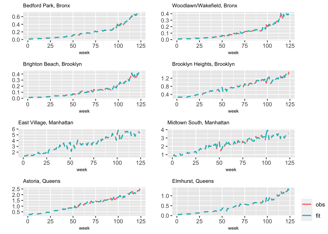
FIGURE 6.2: Observed (red) and fitted (blue) values from Model H1 for eight taxi zones.
In the rest of the chapter, we consider simpler models for TNC usage across zones and over time.
6.3.2 Model H2. Dynamic intercept and Taxi usage
In Model H2, we consider Subway usage and other exogenous variables as fixed effects, setting only the intercept and Taxi usage to be random, dynamic effects. Similar to Model H1, the estimated AR(1) coefficients in the state equations for the intercept and Taxi usage were close to \(1\), so that we show random walk evolutions for these state variables below. The overall level \(\alpha\) is assumed to be a fixed value which is common across the \(g\) zones.
\[\begin{align} Y_{it} &= \alpha + \beta_{it,0}+\beta_{it,1}b_{it,1}+ \beta_{2}b_{it,2}+ \boldsymbol{d}'_{t}\boldsymbol{\gamma}+ \boldsymbol{s}'_{i}\boldsymbol{\eta}+ v_{it}, \notag \\ \beta_{it,0} &= \beta_{i,t-1,0}+w_{it,0}, \notag \\ \beta_{it,1} &= \beta_{i,t-1,1}+w^{(\beta)}_{it,1}. \label{tnc-stbeta-H2} \end{align}\] The formula and model fit are set up as follows.
formula.tnc.H2 <- tnc ~ 1 + subway + holidays + precip +
  median.age + median.earnings + scaled.population + scaled.employment +
  f(id.b0,
    model = "rw1",
    constr = FALSE,
    replicate = re.b0) +
  f(id.taxi,
    taxi,
    model = "rw1",
    constr = FALSE,
    replicate = re.taxi)
model.tnc.H2 <- inla(
  formula.tnc.H2,
  data = ride.data,
  control.predictor = list(compute = TRUE),
  control.compute = list(
    dic = TRUE,
    waic = TRUE,
    cpo = TRUE,
    config = TRUE
  )
)
format.inla.out(model.tnc.H2$summary.fixed[,c(1:5)])
format.inla.out(model.tnc.H2$summary.hyperpar[,c(1:2)])
## name mean sd 0.025q 0.5q 0.975q
## 1 Intercept -2.736 559.697 -1102.662 -2.741 1096.100
## 2 subway 0.002 0.000 0.002 0.002 0.003
## 3 holidays 0.007 0.001 0.005 0.007 0.009
## 4 precip 0.004 0.000 0.003 0.004 0.005
## 5 median.age -0.004 0.005 -0.013 -0.004 0.006
## 6 median.earnings 0.000 0.000 0.000 0.000 0.000
## 7 scaled.population -0.004 0.006 -0.016 -0.004 0.009
## 8 scaled.employment 0.000 0.000 0.000 0.000 0.000
## name mean sd
## 1 Precision for Gaussian obs 1411 52.21
## 2 Precision for id.b0 1096 37.43
## 3 Precision for id.taxi 1252 45.33Among the fixed effects, only Subway usage, holidays, precipitation, and scaled employment (see the result without format.inla.out) are significant. While we only show a few significant digits here, a more complete output can be obtained via summary(model.tnc.H2). Figure 6.3 shows the observed and fitted usage from Model H2 for eight taxi zones.
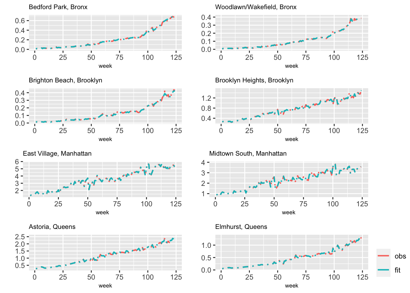
FIGURE 6.3: Observed (red) and fitted (blue) values from Model H2 for eight taxi zones.
In many situations, it may be naive to assume that the level is the same for all zones. To address this, we let the level vary across zones in Model H2, so that the observation equation in Model H2b becomes
\[\begin{align}
Y_{it} &= \alpha_0 + \alpha_i + \beta_{it,0}+\beta_{it,1}b_{it,1}+ \beta_{2}b_{it,2}+
\boldsymbol{d}'_{t}\boldsymbol{\gamma}+
\boldsymbol{s}'_{i}\boldsymbol{\eta}+ v_{it}, \label{tnc-stbeta-H3}
\end{align}\]
while the state equations are the same as under Model H2. We assume that \(\alpha_i \sim N(0, \sigma^2_{\alpha})\), a random effect across the \(g\) zones. Including +1 in the formula below allows us to include an overall fixed level \(\alpha_0\).
formula.tnc.H2b <- tnc ~ 1 + subway + holidays + precip +
  median.age + median.earnings + scaled.population + scaled.employment +
  f(id.alpha, model="iid") +
  f(id.taxi,
    taxi,
    model = "rw1",
    constr = FALSE,
    replicate = re.taxi)
We show a summary of results below. The precision for \(\alpha_i\) is significantly higher than zero, implying that there may be some variation in the level between zones.
format.inla.out(model.tnc.H2b$summary.fixed[,c(1:5)])
format.inla.out(model.tnc.H2b$summary.hyperpar[,c(1,2)])
## name mean sd 0.025q 0.5q 0.975q
## 1 Intercept -3.422 0.214 -3.846 -3.421 -3.005
## 2 subway 0.006 0.001 0.004 0.006 0.007
## 3 holidays -0.007 0.003 -0.012 -0.007 -0.002
## 4 precip 0.015 0.001 0.012 0.015 0.017
## 5 median.age 0.072 0.003 0.065 0.072 0.078
## 6 median.earnings 0.000 0.000 0.000 0.000 0.000
## 7 scaled.population -0.021 0.004 -0.030 -0.021 -0.012
## 8 scaled.employment 0.001 0.000 0.001 0.001 0.001
## name mean sd
## 1 Precision for Gaussian obs 108.368 2.011
## 2 Precision for id.alpha 0.572 0.088
## 3 Precision for id.taxi 531.451 24.098Figure 6.4 shows observed and fitted values from Model H2b.
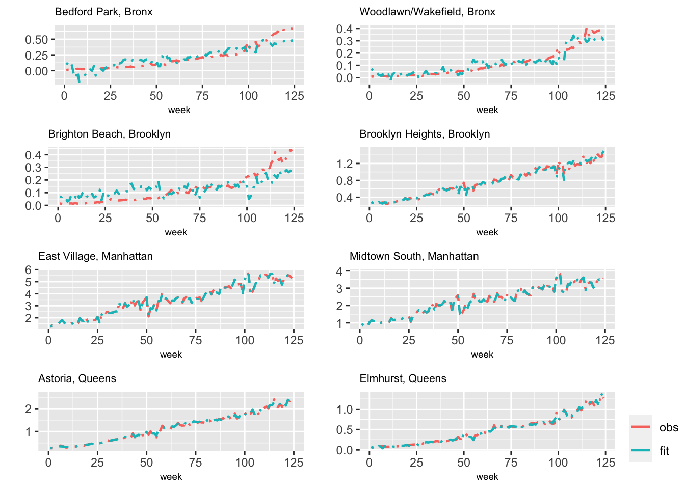
FIGURE 6.4: Observed (red) and fitted (blue) values from Model H2b for eight taxi zones.
Model comparisons are shown in Table 6.1. The data appears to prefer Model H2 as compared with Model H2b. Therefore, we will assume a fixed \(\alpha\) across \(g\) zones in the following models.
Remark. If the number of zones \(g\) was small, we can model the \(\alpha_i\) as fixed effects as shown in the model formula for simulated data in Section 6.2.2, using zone.alpha = as.factor(id.alpha).
6.3.3 Model H3. Taxi usage varies by time and zone
In this model, the intercept is assumed to be a fixed effect and is merged into the level \(\alpha\). Subway usage, median age, median earnings, scaled population, and scaled employment are other fixed effects. Taxi usage is assumed to vary over time and by zone, while holiday, and precipitation are assumed to only vary over time; these effects are modeled by random walks. While we do not show the code and output (see the GitHub page), Figure 6.5 shows the observed and fitted TNC usage from Model H3 for eight taxi zones.
\[\begin{align} Y_{it} &= \alpha + \beta_{it,1}b_{it,1}+ \beta_2 b_{it,2} + \boldsymbol{d}'_{t}\boldsymbol{\gamma}_{t}+ \boldsymbol{s}'_{i}\boldsymbol{\eta_i} + v_{it}, \notag \\ \beta_{it,1} &= \beta_{i,t-1,1}+w^{(\beta)}_{it,1}, \notag \\ \gamma_{t,\ell} &= \gamma_{t-1,\ell}+w^{(\gamma)}_{t,\ell},~\ell=1,2. \label{tnc-stgamma-H3} \end{align}\]
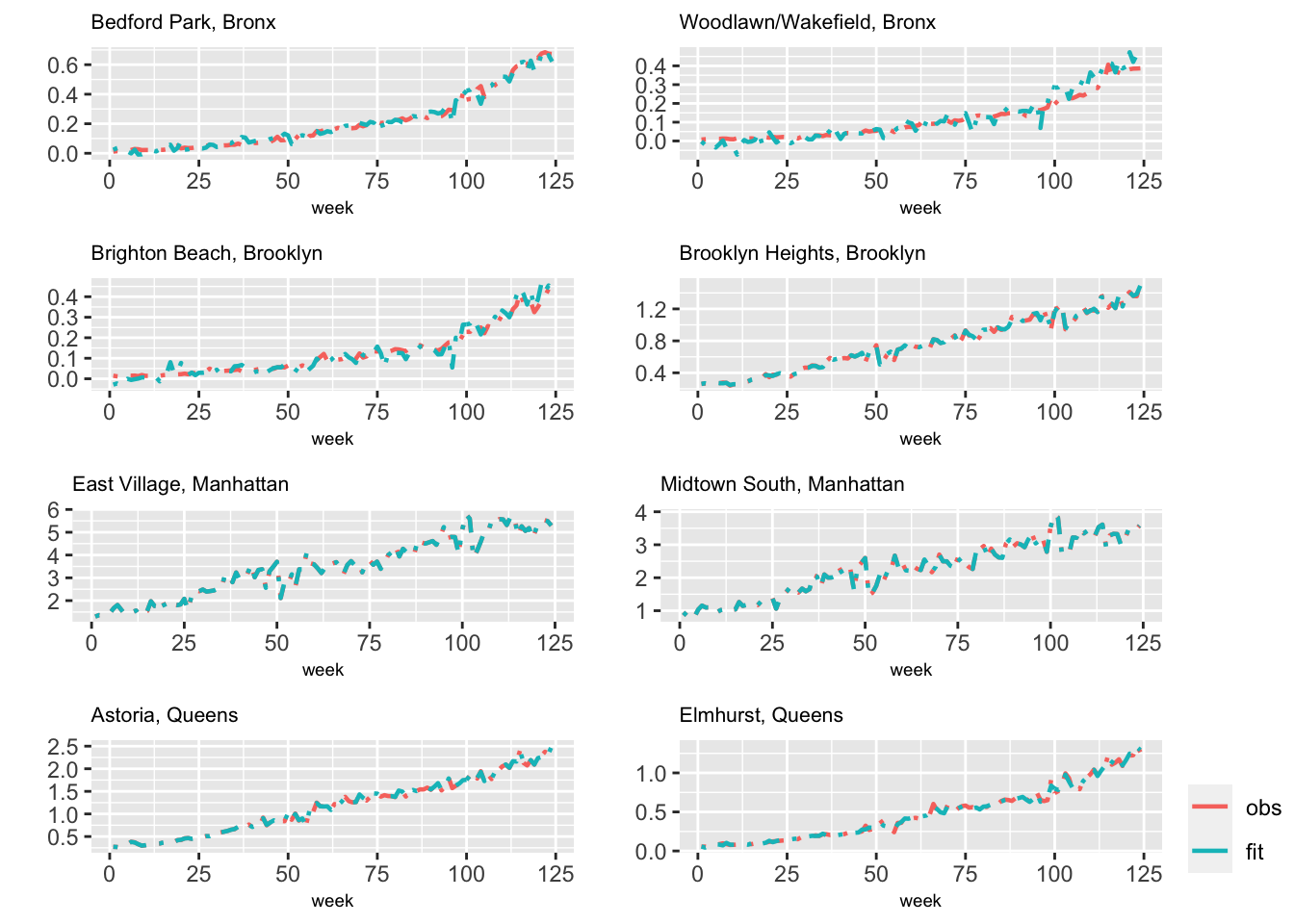
FIGURE 6.5: Observed (red) and fitted (blue) values from Model H3 for eight taxi zones.
6.3.4 Model H4. Fixed intercept, Taxi usage varies over time and zones
Since the results from Model H1 shows high precisions for state errors corresponding to holiday and precipitation, we now treat these variables as static, fixed effects. That is, only Taxi usage varies over time and zones.
\[\begin{align} Y_{it} &= \alpha+\beta_{it,1} b_{it,1}+ \beta_2 b_{it,2}+ \boldsymbol{d}'_{t}\boldsymbol{\gamma}+ \boldsymbol{s}'_{i}\boldsymbol{\eta} + v_{it}, \notag \\ \beta_{it,1} &= \beta_{i,t-1,1}+w^{(\beta)}_{it,1}. \label{tnc-stbeta-H4} \end{align}\]
Figure 6.6 shows the observed and fitted usage from Model H4 for the eight taxi zones.
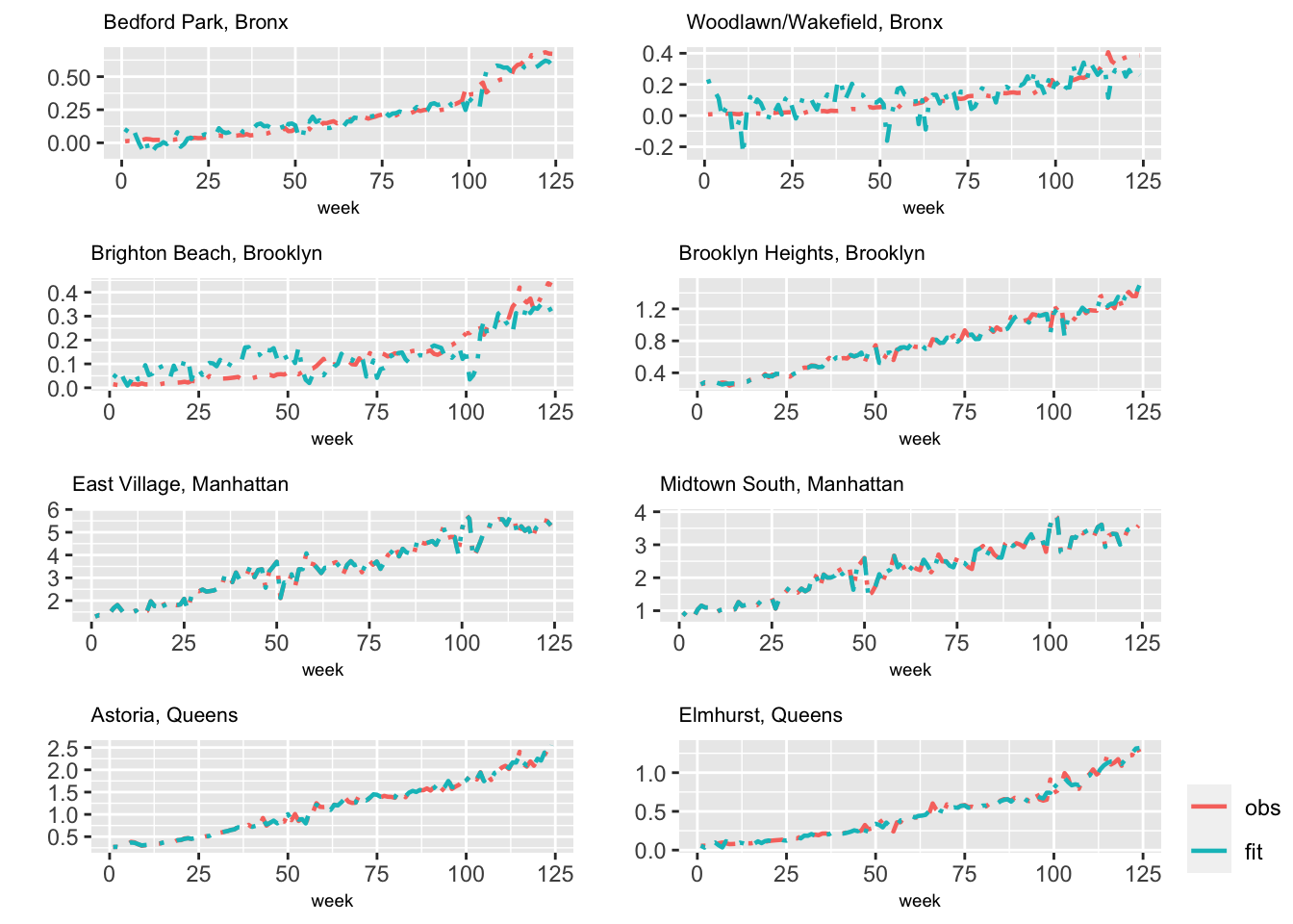
FIGURE 6.6: Observed (red) and fitted (blue) values from Model H4 for eight taxi zones.
6.4 Model comparison
We compare the five models with respect to their in-sample and out of sample performance. In so doing, we first show plots of observed versus fitted values obtained from the five models for a specific zone (Brighton Beach) in Figure 6.7. We also compute and display the in-sample MAPE based on training data for each model for Brighton Beach in Figure 6.7. As suggested from the plot, the MAPE value from Model H1 is the lowest.
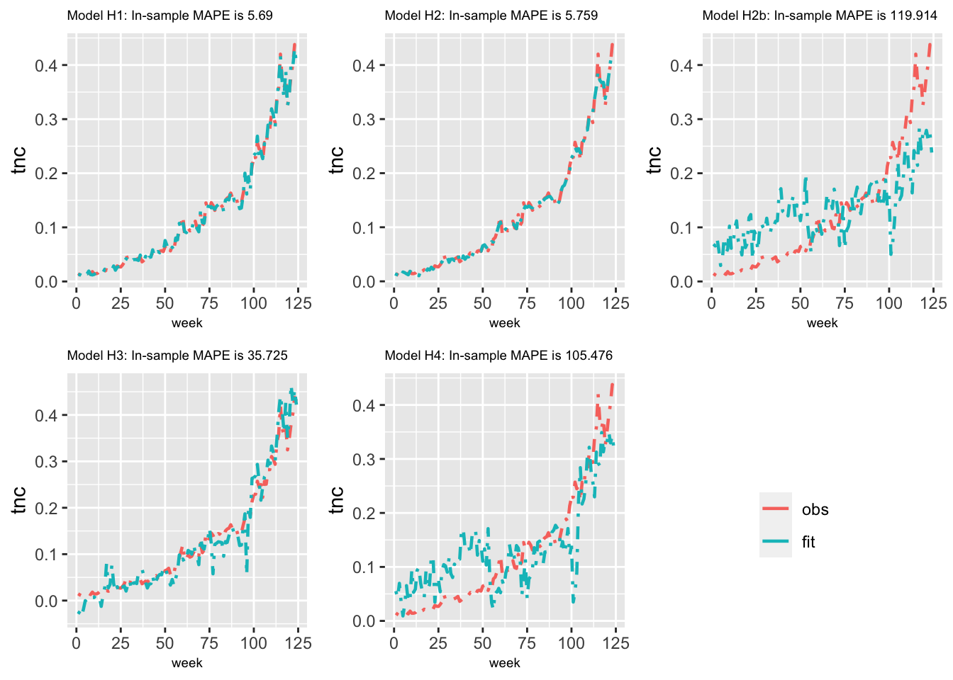
FIGURE 6.7: Plots of observed versus fitted values from all five models for the Brighton Beach taxi zone.
In-sample model comparisons via DIC, WAIC, and PsBF, along with MAE and MAPE across zones are shown in Table 6.1. Note that the MAE (or MAPE) in the table is the average of the MAE (or MAPE) values across zones. The out-of-sample model comparisons via MAE and MAPE (computed based on hold-out data) are shown in Table 6.2. We can also look at the distribution of MAPE and MAE values from all zones and compare models. Figure 6.8 shows boxplots of out-of-sample MAPE values for all zones from the five models; we have suppressed outliers in the boxplots for visual clarity. To see the outliers, set outline = TRUE. The figure shows that the median of MAPE values across zones is lowest from Model H2.
| Model | DIC | WAIC | PsBF | Average in-sample MAE | Average in-sample MAPE |
|---|---|---|---|---|---|
| Model H1 | \(-56232.03\) | \(-56568.628\) | \(106.996\) | \(0.007\) | \(2.798\) |
| Model H2 | \(-51565.851\) | \(-51916.779\) | \(96.177\) | \(0.008\) | \(2.937\) |
| Model H2b | \(-21612.062\) | \(-22698.194\) | \(70.678\) | \(0.046\) | \(40.531\) |
| Model H3 | \(-33653.708\) | \(-35396.272\) | \(12.06\) | \(0.02\) | \(20.346\) |
| Model H4 | \(-21371.145\) | \(-22998.43\) | \(7.905\) | \(0.038\) | \(46.034\) |
| Model | Average out-of-sample MAE | Average out-of-sample MAPE |
|---|---|---|
| Model H1 | 0.021 | 2.635 |
| Model H2 | 0.022 | 1.861 |
| Model H2b | 0.112 | 13.470 |
| Model H3 | 0.060 | 11.318 |
| Model H4 | 0.102 | 12.666 |
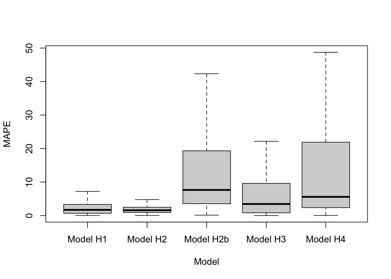
FIGURE 6.8: Boxplots of out-of-sample MAPE values across zones from five models.