Chapter 13 Hierarchical Multivariate Time Series

13.1 Introduction

We describe how R-INLA can be used to fit hierarchical dynamic models for multivariate time series. Section 13.2 extends the Gaussian hierarchical models in Chapter 6 to multivariate (panel) time series, using ideas from Chapter 12. Section 13.3 describes a level correlated model (LCM) for fitting subject-specific models to multiple time series of counts.

Custom functions must be sourced by the user.

source("functions_custom.R")

We use the following packages.

library(mvtnorm)
library(INLA)
library(tidyverse)

We analyze the following data.

1. Ridesourcing in NYC

13.2 Multivariate hierarchical dynamic linear model

Response and predictor variables

For \(t=1,\ldots,n\) and \(i=1,\ldots,g\), let \(\boldsymbol y_{it} = (Y_{1,it}, \ldots, Y_{q,it})'\) denote a \(q\)-dimensional response vector. We can view these \(g\) time series as a panel of vector-valued time series, so that for each \(i\), we have a time series of \(q\)-dimensional vectors, each of length \(n\). The response can be written as a data matrix \(\boldsymbol Y\) with \(g\) rows (subjects/locations) and \(n\) columns (time points), where each element of the matrix is a \(q\)-dimensional vector:

\[\begin{align*} \boldsymbol Y = \begin{pmatrix} \boldsymbol y_{11} & \boldsymbol y_{12} & \ldots & \boldsymbol y_{1n} \\ \boldsymbol y_{21} & \boldsymbol y_{22} & \ldots & \boldsymbol y_{2n} \\ \vdots & \vdots & \ddots & \vdots \\ \boldsymbol y_{g1} & \boldsymbol y_{g2} & \ldots & \boldsymbol y_{gn} \end{pmatrix}. \end{align*}\]

Let \(j=1,\ldots,q\) index the components of \(\boldsymbol y_{it}\). We describe a general framework that involves different types of predictors and corresponding coefficients (similar to Chapter 6).

1. Predictors and coefficients that vary both with time \(t\) and location \(i\): let \(\boldsymbol b_{j,it} = (b_{j,it,1}, \ldots, b_{j,it,c})'\) be a \(c\)-dimensional vector of predictors, and let \(\boldsymbol{\beta}_{j,it}=(\beta_{j,it,1},\ldots,\beta_{j,it,c})'\) be the corresponding location and time-varying coefficient vector.

2. Predictors and coefficients that only vary with time \(t\) and not over locations \(i\): let \(\boldsymbol d_{j,t} = (d_{j,t,1}, \ldots, d_{j,t,a})'\) be an \(a\)-dimensional vector and let \(\boldsymbol{\gamma}_{j,t}=(\gamma_{j,t,1},\ldots,\gamma_{j,t,a})'\) be the corresponding time-varying (or dynamic) coefficient vector.

3. Predictors and coefficients that only vary with location \(i\) and not over time \(t\): suppose that \(\boldsymbol s_{j,i} = (s_{j,i,1}, \ldots, s_{j,i,b})'\) is a \(b\)-dimensional vector and \(\boldsymbol{\eta}_{j,i}=(\eta_{j,i,1},\ldots,\eta_{j,i,b})'\) is the corresponding location specific (or static) coefficient vector.

Note that we can generalize the above setup by allowing \(a\), \(b\), and \(c\) to be \(a_j\), \(b_j\), and \(c_j\) respectively for \(j=1,\ldots,q\), if the data complexity requires this (i.e., we include a different set of predictors for different components of the response vector).

Model setup

A hierarchical dynamic multivariate model for \(\boldsymbol{y}_{it}\) which includes dynamic and static coefficients is shown componentwise for \(j=1,\ldots,q\) as

\[\begin{align} Y_{j,it} & = \alpha_{j,i} + \boldsymbol b'_{j,it}\boldsymbol{\beta}_{j,it} + \boldsymbol d'_{j,t} \boldsymbol{\gamma}_{j,t} + \boldsymbol s'_{j,i}\boldsymbol{\eta}_{j,i} + v_{j,it}, \text{ where}, \tag{13.1} \\ \beta_{j,it,h} & = \phi_j^{(\beta_h)} \beta_{j,i(t-1),h} + w^{(\beta)}_{j,it,h},~h=1,\ldots,c, \tag{13.2} \\ \gamma_{j,t,\ell} & = \phi_j^{(\gamma_\ell)} \gamma_{j,t-1,\ell} + w^{(\gamma_\ell)}_{j,t,\ell},~\ell=1,\ldots,a. \tag{13.3} \end{align}\] In what follows, \(i=1,\ldots,g\) and \(t=1,\ldots,n\). For identifiability, we assume that if an intercept is allowed in the dynamic part, there is no intercept in the static portion, i.e., either \(d_{j,it,1}=1\), or \(s_{j,i,1}=1\). In order to incorporate the dependence between the \(q\) components of \(\boldsymbol y_{it}\), we can assume that

1. the observation error vector \(\boldsymbol v_{it}\) follows a \(q\)-variate normal distribution with mean \(\boldsymbol 0\) and variance \(\boldsymbol V\), for each \(i\) and \(t\),

2. for \(h =1,\ldots, c\), \(\boldsymbol w^{(\beta)}_{it,h}\) follows a \(q\)-variate normal distribution with mean \(\boldsymbol 0\) and variance \(\boldsymbol W^{(\beta_h)}\), for each \(i\) and \(t\), and

3. for \(\ell =1,\ldots, a\), \(\boldsymbol w^{(\gamma)}_{t,\ell}\) follows a \(q\)-variate normal distribution with mean \(\boldsymbol 0\) and variance \(\boldsymbol W^{(\delta_\ell)}\) for each \(t\).

Note that \(\boldsymbol V\), \(\boldsymbol W^{(\beta_h)},~h=1,\ldots,c\), and \(\boldsymbol W^{(\gamma_\ell)},~\ell=1,\ldots,a\) are positive definite (p.d.) covariance matrices. The prior specification for the covariance matrix \(\boldsymbol V\) was discussed in Chapter 12, while the priors for other scalar coefficients were discussed in earlier chapters. We assume an inverse-Wishart prior for \(\boldsymbol V\), i.e., the precision matrix \(\boldsymbol V^{-1}\) follows a Wishart distribution. The iid2d, iid3d, iid4d, and iid5d options enable us to handle these in R-INLA when \(q=2, 3, 4\), or \(5\). State error covariances

\[\begin{align*} & \boldsymbol W^{(\beta_h)}=\text{diag}((\sigma^{(\beta_h)}_{11})^2,\ldots,(\sigma^{(\beta_h)}_{qq})^2),~ h=1,\ldots,c, {\rm and} \\ & \boldsymbol W^{(\gamma_\ell)}=\text{diag}((\sigma^{(\gamma_\ell)}_{11})^2,\ldots,(\sigma^{(\gamma_\ell)}_{qq})^2),~\ell=1,\ldots,a \end{align*}\] are assumed to be diagonal, and we can employ log-gamma priors for the marginal precisions, as discussed in Chapter 3.

13.2.1 Example: Analysis of TNC and Taxi as responses

We build hierarchical Gaussian DLMs similar to Chapter 6 to NYC ridesourcing data, where TNC and Taxi are components of a bivariate response vector \(\boldsymbol{y}_{it} = (Y_{1,it}, Y_{2,it})'\) for zone \(i\) in week \(t\). We again use scaled data for \(n=129\) weeks, but only consider \(g =36\) taxi zones in Manhattan. Figure 13.1 shows time series plots of the scaled (dividing each value by \(10,000\)) TNC and Taxi usage from nine zones in Manhattan.

ride <-
  read.csv("tnc_weekly_data.csv",
           header = TRUE,
           stringsAsFactors = FALSE)
k <- 10000
ride$tnc <- ride$tnc/k
ride$taxi <- ride$taxi/k
ride$subway <- ride$subway/k
# Filter by borough = Manhattan
ride.m <- ride %>%
  filter(borough == "Manhattan")
n <- n_distinct(ride.m$date)
g <- n_distinct(ride.m$zoneid)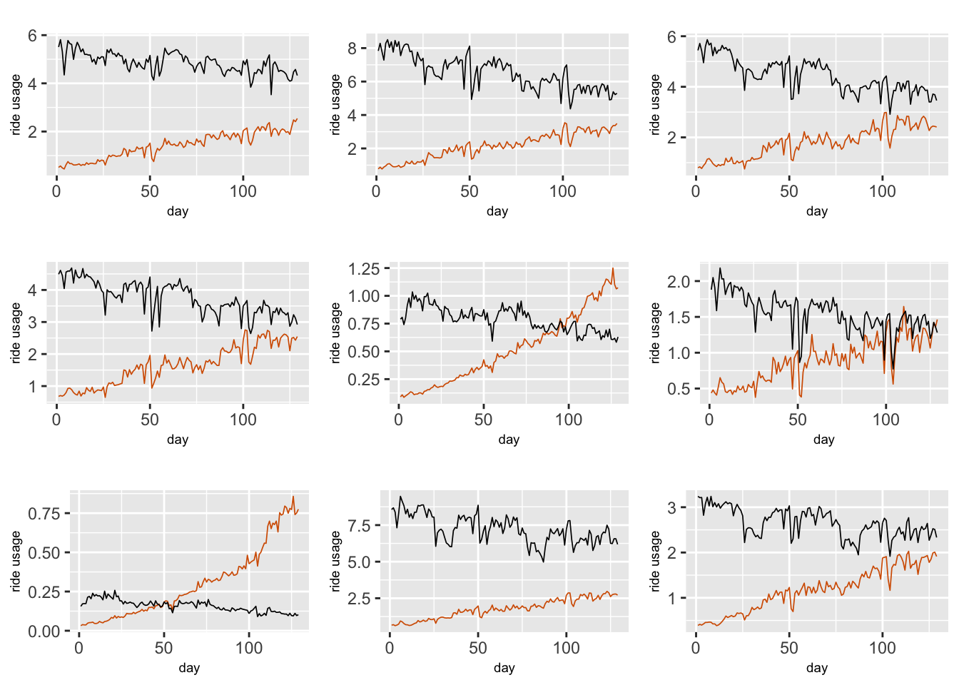

FIGURE 13.1: Weekly scaled TNC (red line) and Taxi (black line) usage in nine different taxi zones in Manhattan.

We reserve data from the last 5 weeks for each zone as hold-out data.

n.hold <- 5
n.train <- n - n.hold
df.zone <- ride.m %>%
  group_split(zoneid, )
test.df <- df.zone %>%
  lapply(function(x)
    tail(x, n.hold)) %>%
  bind_rows()
df.zone.append <- df.zone
for (i in 1:length(df.zone)) {
  df.zone.append[[i]]$tnc[(n.train + 1):n] <- NA
  df.zone.append[[i]]$taxi[(n.train + 1):n] <- NA
}
df.zone.append <- bind_rows(df.zone.append)

We stack the data by zone, while within each zone, we stack the data matrix corresponding to TNC usage followed by a data matrix for Taxi usage, as shown for the multivariate model setup in Chapter 12. We construct subway.tnc and subway.taxi in the following code.

y <- df.zone.append %>%
  group_split(zoneid) %>%
  lapply(function(x)
    unlist(select(x, tnc, taxi))) %>%
  unlist()
subway.tnc <- ride.m %>%
  select(zoneid, subway) %>%
  group_split(zoneid) %>%
  lapply(function(x)
    c(unlist(select(x, subway)), rep(NA, n))) %>%
  unlist()
subway.taxi <- ride.m %>%
  select(zoneid, subway) %>%
  group_split(zoneid) %>%
  lapply(function(x)
    c(rep(NA, n), unlist(select(x, subway)))) %>%
  unlist()

Although we do not show the code, we construct the predictors holidays.tnc and holidays.taxi by replacing “subway” by “holidays” in the code above. Similarly, we construct the predictors precip.tnc and precip.taxi by replacing “subway” by “precip”.

The model is shown below; here \(Y_{1,it}\) and \(Y_{2,it}\) respectively denote TNC usage and Taxi usage.

\[\begin{align} Y_{1,it} = \alpha_{1,i} + \beta_{1,it,0} + \beta_{1,1} Z_{it,1} + \beta_{1,2} Z_{it,2} + \beta_{1,3} Z_{it,3} + v_{1,it}, \notag \\ Y_{2,it} = \alpha_{2,i} + \beta_{2,it,0} + \beta_{2,1} Z_{it,1} + \beta_{2,2} Z_{it,2} + \beta_{2,3} Z_{it,3} + v_{2,it}, \tag{13.4} \end{align}\] with the observation error vector \(\boldsymbol{v}_{it} \sim N(\boldsymbol 0, \boldsymbol V)\), \(\boldsymbol V\) being a \(2 \times 2\) p.d. covariance matrix. The state equation corresponding to the latent vector \(\boldsymbol{\beta}_{it,0} = (\beta_{1,it,0}, \beta_{2,it,0})'\) is

\[\begin{align} \boldsymbol{\beta}_{it,0} = \boldsymbol{\Phi} \boldsymbol{\beta}_{i,t-1,0} + \boldsymbol w_{it}, \tag{13.5} \end{align}\] where \(\boldsymbol w_{it} \sim N(\boldsymbol 0, \boldsymbol W)\), and \(\boldsymbol W\) and \(\boldsymbol{\Phi}\) are assumed to be diagonal. This corresponds to \(q=2\) independent latent AR(1) processes for each zone \(i=1,\ldots, 36\), while \(Z_1, Z_2\), and \(Z_3\) correspond to the predictors Subway usage, holidays, and precipitation. Although we do not do this here, one may also include other predictors such as scaled.population, scaled.employment, median.age, and median.earnings that were discussed in Chapter 6.

Below, we discuss indexes and replicates that are common to Models L1–L3.

N <- 2 * n
t.index <- rep(c(1:N), g)
b0.tnc <- rep(c(1:n, rep(NA, n)), g)
b0.taxi <- rep(c(rep(NA, n), 1:n), g)
re.b0.taxi <- re.b0.tnc <- re.tindex <- rep(1:g, each = N)

Model L1: Same levels for TNC and Taxi usage across all zones

In (13.4), let \(\alpha_{1,i} = \alpha_1\) and \(\alpha_{2,i} = \alpha_2\) for \(i=1,\ldots,g\). The code below sets up the level indexes for this model.

alpha.tnc <- rep(c(rep(1, n), rep(NA, n)), g)
alpha.taxi <- rep(c(rep(NA, n), rep(1, n)), g)

The data is formatted as follows.

tnctaxi.hmv.data <- cbind.data.frame(
  y,
  t.index, re.tindex,
  alpha.tnc, alpha.taxi,
  b0.tnc, re.b0.tnc,
  b0.taxi, re.b0.taxi,
  subway.tnc, subway.taxi,
  holidays.tnc, holidays.taxi,
  precip.tnc, precip.taxi
)

The model formula is shown below, followed by the output.

formula.tnctaxi.hmv <-
  y  ~ -1 + alpha.tnc + alpha.taxi + subway.tnc + subway.taxi +
  holidays.tnc + holidays.taxi + precip.tnc + precip.taxi +
  f(t.index,
    model = "iid2d",
    n = N,
    replicate = re.tindex) +
  f(b0.tnc,
    model = "rw1",
    constr = FALSE,
    replicate = re.b0.tnc) +
  f(b0.taxi,
    model = "rw1",
    constr = FALSE,
    replicate = re.b0.taxi)

model.tnctaxi.hmv <-
  inla(
    formula.tnctaxi.hmv,
    family = c("gaussian"),
    data = tnctaxi.hmv.data,
    control.inla = list(h = 1e-5,
                        tolerance = 1e-3),
    control.compute = list(
      dic = TRUE,
      waic = TRUE,
      cpo = TRUE,
      config = TRUE
    ),
    control.predictor = list(compute = TRUE),
    control.family =
      list(hyper = list(prec = list(
        initial = 10,
        fixed = TRUE
      ))),
  )

Posterior summaries for the fixed and random effects are shown below. The observation error correlation \(R_{12}\) is significant, with a posterior mean of 0.776. The estimated \(\alpha_1\) and \(\alpha_2\) for TNC and Taxi usage are very close to zero. In the next section, we will investigate a model with different levels for TNC and Taxi usage for the different zones.

format.inla.out(model.tnctaxi.hmv$summary.fixed[,c(1,2,4)])
##   name          mean  sd     0.5q 
## 1 alpha.tnc     0.001 31.626 0.000
## 2 alpha.taxi    0.001 31.626 0.000
## 3 subway.tnc    0.029  0.001 0.029
## 4 subway.taxi   0.064  0.001 0.064
## 5 holidays.tnc  0.024  0.006 0.024
## 6 holidays.taxi 0.028  0.013 0.028
## 7 precip.tnc    0.035  0.003 0.035
## 8 precip.taxi   0.008  0.006 0.008
format.inla.out(model.tnctaxi.hmv$summary.hyperpar[,c(1,2,4,5)])
##   name                              mean    sd     0.5q    0.975q 
## 1 Precision for t.index component 1  57.975  1.821  57.940  61.654
## 2 Precision for t.index component 2  13.565  0.391  13.557  14.355
## 3 Rho1:2 for t.index                  0.776  0.009   0.776   0.793
## 4 Precision for b0.tnc              178.985 10.500 178.601 200.638
## 5 Precision for b0.taxi              56.613  3.372  56.492  63.553

Fitted values and forecasts

Similar to Approach 1 in Chapter 12, we obtain fitted values and forecasts through posterior samples of the model parameters and hyperparameters using inla.posterior.sample(). We create a custom function fit.post.sample.hmv().

fit.post.sample.hmv <- function(x) {
  set.seed(123457)
  sigma2.v1 <- 1 / x$hyperpar[1]
  sigma2.v2 <- 1 / x$hyperpar[2]
  rho.v1v2 <- x$hyperpar[3]
  cov.v1v2 <- rho.v1v2 * sqrt(sigma2.v1) * sqrt(sigma2.v2)
  sigma.v <-
    matrix(c(sigma2.v1, cov.v1v2, cov.v1v2, sigma2.v2), nrow = 2)
  b0.tnc <-
    matrix(x$latent[grep("b0.tnc", rownames(x$latent))], nrow = n)
  b0.taxi <-
    matrix(x$latent[grep("b0.taxi", rownames(x$latent))], nrow = n)
  fit.tnc <- fit.taxi <- vector("list", n)
  for (j in 1:g) {
    V <- rmvnorm(n, mean = c(0, 0), sigma = sigma.v)
    V1 <- V[, 1]
    V2 <- V[, 2]
    fit.tnc[[j]] <-
      x$latent[grep("alpha.tnc", rownames(x$latent))] +
      b0.tnc[, j] +
      x$latent[grep("subway.tnc", rownames(x$latent))] *
      df.zone[[j]]$subway +
      x$latent[grep("holidays.tnc", rownames(x$latent))] *
      df.zone[[j]]$holidays +
      x$latent[grep("precip.tnc", rownames(x$latent))] *
      df.zone[[j]]$precip +
      V1
    fit.taxi[[j]] <-
      x$latent[grep("alpha.taxi", rownames(x$latent))] +
      b0.taxi[, j] +
      x$latent[grep("subway.taxi", rownames(x$latent))] *
      df.zone[[j]]$subway +
      x$latent[grep("holidays.taxi", rownames(x$latent))] *
      df.zone[[j]]$holidays +
      x$latent[grep("precip.taxi", rownames(x$latent))] *
      df.zone[[j]]$precip +
      V2
  }
  fit.tnc <-
    bind_cols(fit.tnc,
              .name_repair = ~ vctrs::vec_as_names(names =
                                                     paste0("g", 1:g)))
  fit.taxi <-
    bind_cols(fit.taxi,
              .name_repair = ~ vctrs::vec_as_names(names =
                                                     paste0("g", 1:g)))
  return(list(fit.tnc = fit.tnc, fit.taxi = fit.taxi))
}

The fitted values for scaled TNC and Taxi usage for each zone are computed by calling this function. Here, we demonstrate the computation for one zone (zoneid = “ID100”). The plots of observed and fitted and forecast values are shown in Figure 13.2.

fits <- post.sample.hmv %>%
  mclapply(function(x)
    fit.post.sample.hmv(x))
zone <- match("ID100", unique(df.zone.append$zoneid))
tnc.fit <- fits %>%
  lapply(function(x)
    x$fit.tnc[, zone]) %>%
  bind_cols() %>%
  rowMeans()
taxi.fit <- fits %>%
  lapply(function(x)
    x$fit.taxi[, zone]) %>%
  bind_cols() %>%
  rowMeans()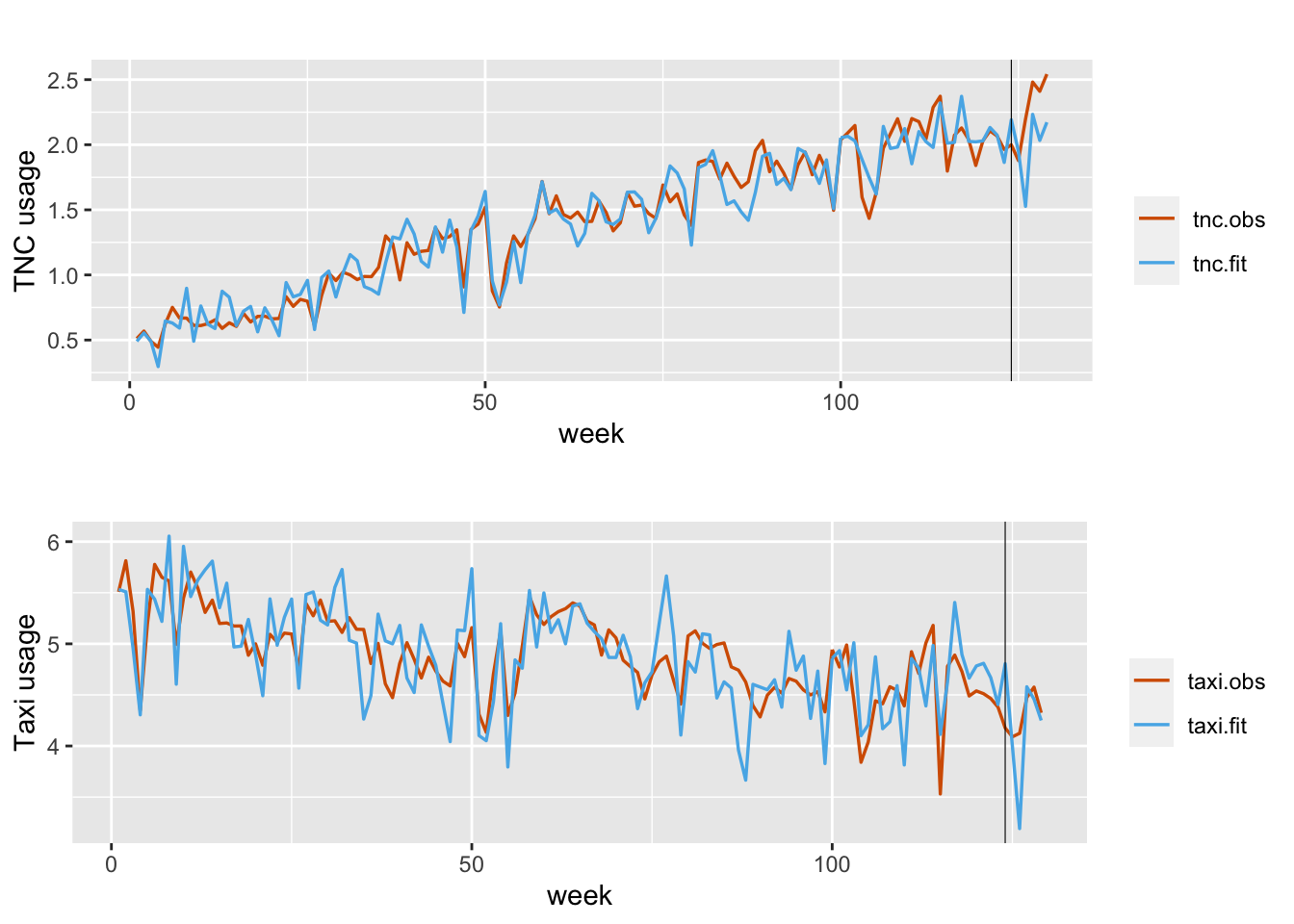

FIGURE 13.2: Observed (red) and fitted (blue) TNC (top plot) and Taxi usage for zone ID100 under Model L1. The black vertical line divides the data into training and test portions.

Model L2. Different fixed-effect zone-specific levels

We consider zone-specific levels \(\alpha_{j,i},~j=1,2\) in (13.4). For a model with different fixed levels across zones, the indexes for \(\alpha_{j,i}\) are defined below.

id.alpha.tnc <- id.alpha.taxi <- c()
for (i in 1:g) {
  temp.tnc <- c(rep(i, n), rep(NA, n))
  id.alpha.tnc <- c(id.alpha.tnc, temp.tnc)
  temp.taxi <- c(rep(NA, n), rep(i, n))
  id.alpha.taxi <- c(id.alpha.taxi, temp.taxi)
}
fact.alpha.tnc <- as.factor(id.alpha.tnc)
fact.alpha.taxi <- as.factor(id.alpha.taxi)

To get the formatted data tnctaxi.hmvfe.data for Model L1, we replace alpha.tnc and alpha.taxi by fact.alpha.tnc and fact.alpha.taxi in tnctaxi.hmv.data. The model formula formula.tnctaxi.hmvfe is the same as formula.tnctaxi.hmv except for replacing

y ~ -1 + alpha.tnc + alpha.taxi + subway.tnc +...

by

y ~ -1 + fact.alpha.tnc + fact.alpha.taxi + subway.tnc+...

We change the code

model.tnctaxi.hmv <-
  inla(
    formula.tnctaxi.hmv,
    family = c("gaussian"),
    data = tnctaxi.hmv.data, ...

in Model L1 to

model.tnctaxi.hmvfe <-
  inla(
    formula.tnctaxi.hmvfe,
    family = c("gaussian"),
    data = tnctaxi.hmvfe.data, ...

and obtain the following results.

##   name          mean  sd    0.5q 
## 1 subway.tnc    0.029 0.001 0.029
## 2 subway.taxi   0.064 0.001 0.064
## 3 holidays.tnc  0.024 0.006 0.024
## 4 holidays.taxi 0.028 0.013 0.028
## 5 precip.tnc    0.035 0.003 0.035
## 6 precip.taxi   0.008 0.006 0.008
##   name                              mean    sd     0.025q  0.975q 
## 1 Precision for t.index component 1  58.030  1.817  54.531  61.681
## 2 Precision for t.index component 2  13.573  0.397  12.807  14.371
## 3 Rho1:2 for t.index                  0.775  0.009   0.757   0.793
## 4 Precision for b0.tnc              178.705 10.325 159.478 199.958
## 5 Precision for b0.taxi              56.660  3.435  50.271  63.746

The posterior means for all the \(\alpha_{j,i}\) are not significantly different than zero. The estimates of the other fixed effects and random effects are very similar to estimates from Model L1. The estimated correlation \(R_{12}\) is about 0.775. Under Model L1, we defined the custom function fit.post.sample.hmv() which uses inla.posterior.sample(). Here, we can use the same function to compute the fitted values with some minor changes, details of which are available on our GitHub link.

Model L3. Different random-effect zone-specific levels

We assume that \(\alpha_{j,i} \sim N(0, \sigma^2_j)\) for \(i=1,\ldots,g\). The indexes for the random \(\alpha_{j,i}\) are computed as follows.

id.alpha.tnc <- id.alpha.taxi <- c()
for (i in 1:g) {
  temp.tnc <- c(rep(i,n), rep(NA, n))
  id.alpha.tnc <- c(id.alpha.tnc, temp.tnc)
  temp.taxi <- c(rep(NA, n), rep(i, n))
  id.alpha.taxi <- c(id.alpha.taxi, temp.taxi)
}

The formatted data tnctaxi.hmvre.data is constructed by replacing alpha.tnc and alpha.taxi in tnctaxi.hmv.data under Model L1 by id.alpha.tnc and id.alpha.taxi.

The model formula is given below.

prec.prior <- list(prec = list(param = c(0.001, 0.001)))
formula.tnctaxi.hmvre <-
  y  ~ -1 + 
  f(id.alpha.tnc, model = "iid", hyper = prec.prior) +
  f(id.alpha.taxi, model = "iid", hyper = prec.prior) +
  subway.tnc + subway.taxi + holidays.tnc + holidays.taxi +
  precip.tnc + precip.taxi +
  f(t.index,
    model = "iid2d",
    n = N,
    replicate = re.tindex) +
  f(b0.tnc,
    model = "rw1",
    constr = FALSE,
    replicate = re.b0.tnc) +
  f(b0.taxi,
    model = "rw1",
    constr = FALSE,
    replicate = re.b0.taxi)

We obtain results by changing the code for Model L1 from

model.tnctaxi.hmv <-
  inla(
    formula.tnctaxi.hmv,
    family = c("gaussian"),
    data = tnctaxi.hmv.data, ...

to the code below:

model.tnctaxi.hmvre <-
  inla(
    formula.tnctaxi.hmvre,
    family = c("gaussian"),
    data = tnctaxi.hmvre.data, ...

##   name          mean  sd    0.5q 
## 1 subway.tnc    0.029 0.001 0.029
## 2 subway.taxi   0.064 0.001 0.064
## 3 holidays.tnc  0.024 0.006 0.024
## 4 holidays.taxi 0.028 0.013 0.028
## 5 precip.tnc    0.035 0.003 0.035
## 6 precip.taxi   0.008 0.006 0.008
##   name                              mean    sd     0.5q    0.975q 
## 1 Precision for id.alpha.tnc         63.743 44.756  51.855 184.685
## 2 Precision for id.alpha.taxi        79.883 73.026  58.269 277.321
## 3 Precision for t.index component 1  58.014  1.836  57.986  61.696
## 4 Precision for t.index component 2  13.571  0.396  13.565  14.364
## 5 Rho1:2 for t.index                  0.775  0.010   0.776   0.794
## 6 Precision for b0.tnc              178.962 10.523 178.623 200.622
## 7 Precision for b0.taxi              56.701  3.440  56.596  63.766

The fitted values are computed using inla.posterior.sample()and the function fit.sample.hmv.re(). For details, see the GitHub link for the book.

In-sample and out-of-sample model comparisons for the three models are shown in Table 13.1. The DIC, WAIC, and MAE values (averaged over all zones) are similar across the three models. The simplest model is Model L1.

TABLE 13.1: Comparison of Models L1–L3.

Model	DIC	WAIC	Average Out-of-Sample MAE (TNC)	Average Out-of-Sample MAE(Taxi)
L1	\(-55035.97\)	\(-57758.129\)	\(0.222\)	\(0.336\)
L2	\(-55035.969\)	\(-57758.148\)	\(0.178\)	\(0.223\)
L3	\(-55035.963\)	\(-57758.201\)	\(0.176\)	\(0.228\)

13.3 Level correlated models for multivariate time series of counts

In certain situations, we need to build a model for a multivariate time series of counts as a function of its history and available exogenous predictors. The dependence between the components may be due to omitted variables which simultaneously affect the response vector (Aitchison and Ho (1989); Chib and Winkelmann (2001)). Univariate count (Poisson or negative binomial) models for each component cannot account for the dependence among the components. See Refik Soyer and Zhang (2021) for a detailed review of general ideas in Bayesian modeling of multivariate time series of counts.

Serhiyenko, Ravishanker, and Venkatesan (2018) described level correlated models (LCMs) which allow us to combine different component count distributions, accommodate their dependence, and offer a flexible modeling approach using R-INLA; also see Serhiyenko (2015) and Serhiyenko, Ravishanker, and Venkatesan (2015). Serhiyenko et al. (2016) and K. Wang et al. (2017) discussed crash counts modeling in transportation safety. B. Raman et al. (2021) presented a application in marketing to assess effectiveness of promotions on product sales, while Y. Wang, Zou, and Ravishanker (2021) described an application for high-frequency financial data.

Let \(\boldsymbol{y}_{it}=(y_{1,it}, \ldots, y_{q,it})'\) be a \(q\)-variate vector of count responses over time, for \(i=1,\ldots,g\) and \(t=1,\ldots,n\). That is, we observe \(q\) components of counts on \(g\) subjects (or at \(g\) locations) over \(n\) regularly spaced time points. As shown in Serhiyenko, Ravishanker, and Venkatesan (2018) or B. Raman et al. (2021), we can write the LCM for the multivariate count time series as a state space model. In the following, \(i=1,\ldots,g\), \(t=1,\ldots,n\), and \(j=1,\ldots,q\).

13.3.1 Example: TNC and Taxi counts based on daily data

We look at daily TNC and Taxi counts over 3 years from 34 zones in Manhattan.

ride.m <-
  read.csv(
    "tnctaxi_daily_data_Manhattan.csv",
    header = TRUE,
    stringsAsFactors = FALSE
  )
n <- n_distinct(ride.m$date)
g1 <- n_distinct(ride.m$zoneid)

We hold out 14 days (two weeks) of data and set up the training and test data as follows.

n.hold <- 14 # 2 weeks
n.train <- n - n.hold
df.zone <- ride.m %>%
  group_split(zoneid)
test.df <- df.zone %>%
  lapply(function(x)
    tail(x, n.hold)) %>%
  bind_rows()
df.zone.append <- df.zone
for (i in 1:length(df.zone)) {
  df.zone.append[[i]]$tnc[(n.train + 1):n] <- NA
  df.zone.append[[i]]$taxi[(n.train + 1):n] <- NA
}
df.zone.append <- bind_rows(df.zone.append)

Model LCM1 for TNC and Taxi counts

Similar to Model Z1 in Chapter 9, we include zone-specific fixed levels \(\alpha_{j,i}\) for each type \(j\), a linear trend \(\gamma t\), and fixed effects corresponding to the predictors \(\cos(2 \pi t/7)\) and \(\sin(2 \pi t/7)\) (to handle the seasonality with period \(7\)), and Subway usage. We denote these predictors by \(Z_{t,\ell},~\ell=1,\ldots,3\). We include a dynamic intercept \(\beta_{j,it,0}\) (this was denoted by \(X_{j, it}\) in the general specification above) which is modeled as a random walk. We assume that the level correlated effect \(\boldsymbol{\xi} = (\xi_{1,it}, \xi_{2,it})' \sim N(\boldsymbol{0}, \boldsymbol{\Sigma})\). The model is

\[\begin{align} Y_{j,it}| \lambda_{j,it} &\sim \text{UDC}_j(\lambda_{j,it}), \notag \\ \log \lambda_{j,it} &= \alpha_{j,i} + \gamma t + \beta_{j,it,0} + \sum_{\ell=1}^3 \beta_\ell Z_{t,\ell} + \xi_{j,it}, \notag \\ \beta_{j,it,0} & = \beta_{j,i,t-1,0}+ w_{j,it}, \tag{13.6} \end{align}\] where \(w_{j,it}\) is N\((0, \sigma^2_{j})\). The indexes and replicates are constructed in the code below.

N <- 2 * n
trend <- rep(1:n, 2)
htrend <- rep(trend, g1)
seas.per <- 7
costerm <- cos(2 * pi * trend / seas.per)
sinterm <- sin(2 * pi * trend / seas.per)
hcosterm <- rep(costerm, g1)
hsinterm <- rep(sinterm, g1)
#indexes
t.index <- rep(c(1:N), g1)
b0.tnc <- rep(c(1:n, rep(NA, n)), g1)
b0.taxi <- rep(c(rep(NA, n), 1:n), g1)
## replicates
re.b0.taxi <- re.b0.tnc <- re.tindex <- rep(1:g1, each = N)
id.alpha.tnc <- rep(1:g1, each = N)
fact.alpha.tnc <- as.factor(id.alpha.tnc)
id.alpha.taxi <- rep(1:g1, each = N)
fact.alpha.taxi <- as.factor(id.alpha.taxi)

The following code shows how to set up the predictor Subway usage corresponding to the TNC and Taxi counts.

y <- df.zone.append %>%
  group_split(zoneid) %>%
  lapply(function(x)
    unlist(select(x, tnc, taxi))) %>%
  unlist()
subway.tnc <- ride.m %>%
  select(zoneid, subway) %>%
  group_split(zoneid) %>%
  lapply(function(x)
    c(unlist(select(x, subway)), rep(NA, n))) %>%
  unlist()
subway.taxi <- ride.m %>%
  select(zoneid, subway) %>%
  group_split(zoneid) %>%
  lapply(function(x)
    c(rep(NA, n), unlist(select(x, subway)))) %>%
  unlist()

We collect the variables into a data frame data.ride.lcm1.

data.ride.lcm1 <-cbind.data.frame(y, t.index, htrend, hcosterm, hsinterm, 
                                  fact.alpha.tnc, fact.alpha.taxi,
                                  b0.tnc, b0.taxi, 
                                  re.b0.tnc, re.b0.taxi, re.tindex,  
                                  subway.tnc, subway.taxi)

We assume Poisson observation models for both TNC and Taxi counts; i.e., we set UDC as Poisson. We set up the formula by assuming that the levels \(\alpha_{j,i}\) are fixed effects, and use default prior specifications. The results are summarized below. Detailed output can be obtained from our GitHub link.

formula.ride.lcm1 <-
  y ~ -1 + fact.alpha.tnc + fact.alpha.taxi + 
  htrend + hcosterm + hsinterm + 
  subway.tnc + subway.taxi +
  f(t.index,
    model = "iid2d",
    n = N,
    replicate = re.tindex) +
  f(b0.tnc,
    model = "rw1",
    constr = FALSE,
    replicate = re.b0.tnc) +
  f(b0.taxi,
    model = "rw1",
    constr = FALSE,
    replicate = re.b0.taxi)

model.pois.lcm1 <- inla(formula.ride.lcm1,
      data = data.ride.lcm1,
      family="poisson",
      control.inla = list(h = 1e-5, tolerance = 1e-3),
      control.predictor = list(compute = TRUE, link = 1),
      control.compute = list(dic = TRUE, waic = TRUE, 
                             cpo = TRUE, config = TRUE),
      control.fixed = list(expand.factor.strategy = "inla")
      )
summary.model.pois.lcm1 <- summary(model.pois.lcm1)

#format.inla.out(head(summary.model.pois.lcm1$fixed[,c(1,2, 5)]))
format.inla.out(summary.model.pois.lcm1$hyperpar[,c(1,2)])
##   name                              mean     sd     
## 1 Precision for t.index component 1    64.29   1.711
## 2 Precision for t.index component 2    66.01   1.165
## 3 Rho1:2 for t.index                    0.92   0.003
## 4 Precision for b0.tnc               3924.43 241.019
## 5 Precision for b0.taxi             10183.25 838.265

Posterior means for the levels \(\alpha_{j,i}\) are very small (\(<1e-05\)). The details can be obtained by using model.pois.lcm1$summary.fixed.

We use inla.posterior.sample() to generate posterior samples of model parameters and hyperparameters, and construct distributions of fitted responses. Figure 13.3 shows plots of observed and fitted TNC and Taxi counts in zone ID107.

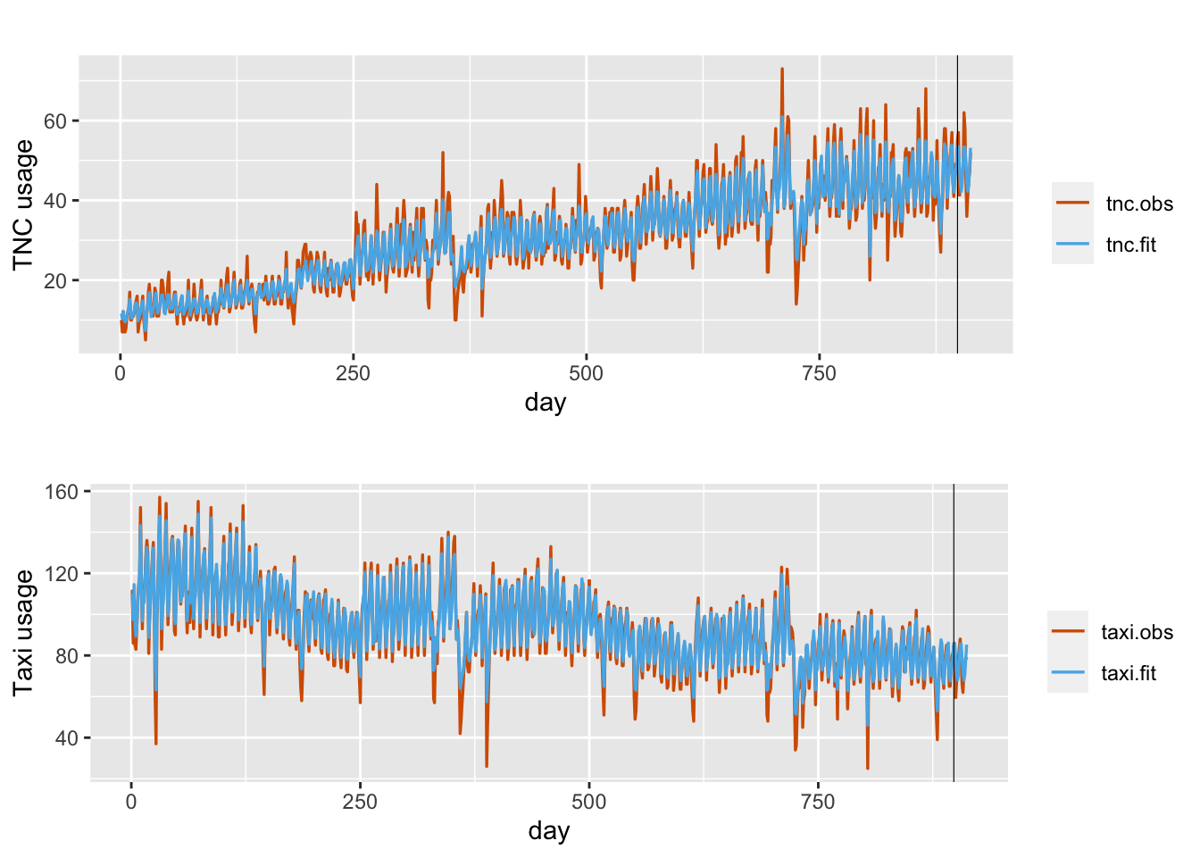
FIGURE 13.3: Observed (red) and fitted(blue) daily TNC and Taxi counts in taxi zone ID107 under Model LCM1. The black vertical line divides the data into training and test portions.

Since this setup involves likelihoods of two components, we can alternatively set up the responses in a matrix form and modify the formula and inla() call. Specifically, we replace

y <- df.zone.append %>% 
  group_split(zoneid) %>% 
  lapply(function(x) unlist(select(x, tnc, taxi))) %>% 
  unlist()

in the code above by

y <- df.zone.append %>% 
  group_split(zoneid) %>% 
  lapply(function(x) unlist(select(x, tnc, taxi))) %>% 
  unlist()
y.alt.tnc <- df.zone.append %>% 
  group_split(zoneid) %>% 
  lapply(function(x) c(x$tnc, rep(NA, n))) %>% 
  unlist()
y.alt.taxi <- df.zone.append %>% 
  group_split(zoneid) %>% 
  lapply(function(x) c(rep(NA, n), x$taxi)) %>% 
  unlist()
Y <- matrix(c(y.alt.tnc, y.alt.taxi), ncol = 2)

We also replace y by Y in the data frame and formula. It can be verified that this code produces exactly the same results as the previous code. More details are given in our GitHub link.

model.pois.pois.lcm1 <- inla(
  formula.ride.lcm1,
  data = data.ride.lcm1,
  family = c("poisson", "poisson"),
  control.inla = list(h = 1e-5,
                      tolerance = 1e-3),
  control.predictor = list(compute = TRUE),
  control.compute = list(dic = TRUE, waic = TRUE, cpo = TRUE),
)

Based on the results, the Poisson distribution seems to be a good fit to the TNC and Taxi usage data. However, in other examples, count data may exhibit overdispersion and/or zero-inflation. R-INLA includes the negative binomial and zero-inflated Poisson as other options for observation models for counts. These can be invoked via family = c("nbinomial") or family = c("zeroinflatedpoisson1"). If all the components are assumed to follow the same UDC, then we can use the first code or the alternate code shown under Model LCM1. However, if the components follow different distributions, the alternate code (which uses the matrix \(Y\) instead of the vector \(y\)) must be used. For example, we can include family = c("nbinomial", "poisson") to assume that UDC is negative binomial for the first component and Poisson for the second component. Since neither the negative binomial nor the zero-inflated Poisson are suitable distributions for TNC or Taxi counts, we do not illustrate these here. See Serhiyenko, Ravishanker, and Venkatesan (2018) for the use of different UDC’s with an application to marketing data.

Next, we consider a different model for TNC and Taxi counts instead of Model LCM1.

Model LCM2 for TNC and Taxi counts

We assume that the dynamic random effect or the levels do not vary by zone \(i\). That is, \(\alpha_{j,i} = \alpha_j\) and \(\beta_{j,it,0} = \beta_{j,t,0}\) for all \(i\).

\[\begin{align} Y_{j,it}| \lambda_{j,it} &\sim \text{UDC}_j(\lambda_{j,it}), \notag \\ \log \lambda_{j,it} &= \alpha_j + \gamma_j t + \beta_{j,t,0} + \sum_{\ell=1}^3 \beta_\ell Z_{t,\ell} + \xi_{j,it}, \notag \\ \beta_{j,t,0} &= \beta_{j,t-1,0}+ w_{j,t,0}, \tag{13.7} \end{align}\] where \(w_{j,t}\) is N\((0, \sigma^2_{w})\). Let UDC be the Poisson distribution. We again read in the daily data from 34 zones in Manhattan and set up the training and test sets. The indexes and replicates are shown below.

N <- 2 * n
trend <- rep(1:n, 2)
htrend <- rep(trend, g1)
seas.per <- 7
costerm <- cos(2 * pi * trend / seas.per)
sinterm <- sin(2 * pi * trend / seas.per)
hcosterm <- rep(costerm, g1)
hsinterm <- rep(sinterm, g1)
#indexes
t.index <- rep(c(1:N), g1)
b0.tnc <- id.re.b0.tnc <- rep(c(1:n, rep(NA, n)), g1)
b0.taxi <- id.re.b0.taxi <- rep(c(rep(NA, n), 1:n), g1)
## replicates
re.tindex <- rep(1:g1, each = N)
re.b0.taxi <- re.b0.tnc <- rep(rep(c(1, 2), each = n), each = g1)
id.alpha.tnc <- rep(1:g1, each = N)
fact.alpha.tnc <- as.factor(id.alpha.tnc)
id.alpha.taxi <- rep(1:g1, each = N)
fact.alpha.taxi <- as.factor(id.alpha.taxi)

We then set up the data frame.

y <- df.zone.append %>% 
  group_split(zoneid) %>% 
  lapply(function(x) unlist(select(x, tnc, taxi))) %>% 
  unlist()
subway.tnc <- ride.m %>% 
  select(zoneid, subway) %>% 
  group_split(zoneid) %>% 
  lapply(function(x) c(unlist(select(x,subway)), rep(NA, n))) %>% 
  unlist()
subway.taxi <- ride.m %>% 
  select(zoneid, subway) %>% 
  group_split(zoneid) %>% 
  lapply(function(x) c(rep(NA, n),unlist(select(x,subway)))) %>% 
  unlist()
data.ride.lcm2 <-cbind.data.frame(y, t.index, htrend, hcosterm, hsinterm, 
                                  id.alpha.tnc, id.alpha.taxi,
                                  b0.tnc, b0.taxi, 
                                  re.b0.tnc, re.b0.taxi, re.tindex,  
                                  subway.tnc, subway.taxi,
                                  id.re.b0.tnc, id.re.b0.taxi)

The formula and model output are shown below.

formula.ride.lcm2 <-
  y ~ -1 + fact.alpha.tnc + fact.alpha.taxi +
  htrend + hcosterm + hsinterm + 
  subway.tnc + subway.taxi +
  f(t.index,
    model = "iid2d",
    n = N,
    replicate = re.tindex) +
  f(b0.tnc,
    model = "rw1",
    constr = FALSE) +
  f(id.re.b0.tnc, model = "iid",
    replicate = re.b0.tnc, 
    hyper = list(prec=list(fixed=T, initial = 20))) +
  f(b0.taxi,
    model = "rw1",
    constr = FALSE) +
  f(id.re.b0.taxi, model="iid", 
    replicate = re.b0.taxi,
    hyper = list(prec=list(fixed=T, initial = 20)))

##   name       mean   sd     0.975q
## 1 alpha.tnc   0.000 31.622 62.033
## 2 alpha.taxi -0.001 31.618 62.024
## 3 htrend      0.000  0.001  0.001
## 4 hcosterm   -0.101  0.006 -0.089
## 5 hsinterm    0.099  0.006  0.110
## 6 subway.tnc  0.004  0.000  0.004

##   name                              mean     sd     
## 1 Precision for t.index component 1    3.554   0.028
## 2 Precision for t.index component 2    1.739   0.012
## 3 Rho1:2 for t.index                   0.949   0.001
## 4 Precision for b0.tnc               235.549  34.807
## 5 Precision for b0.taxi             2976.154 877.149

Plots of the observed and fitted responses are shown in Figure 13.4.

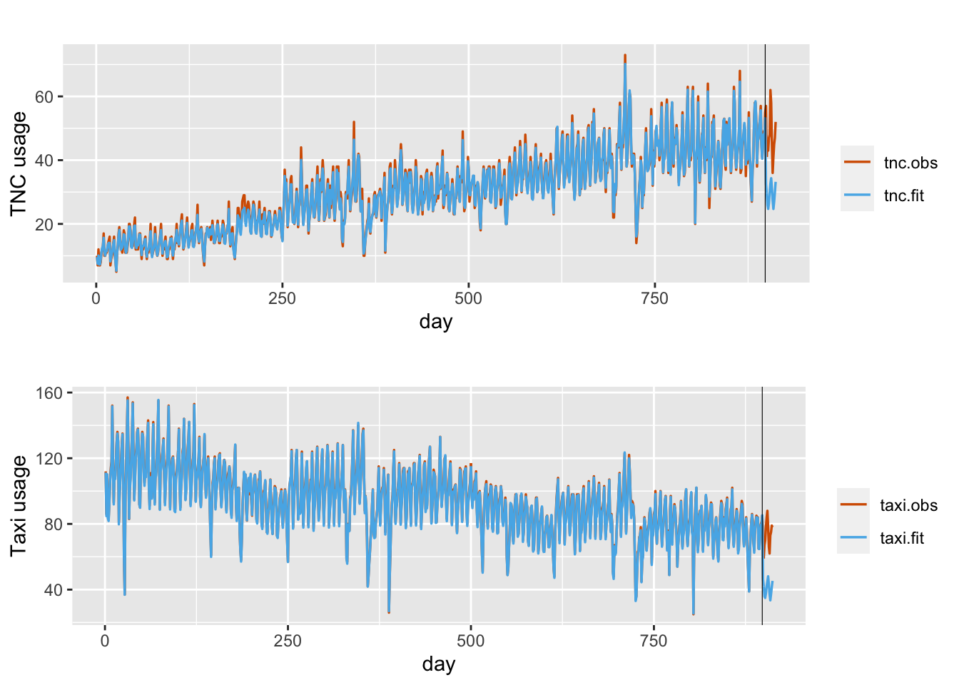
FIGURE 13.4: Observed (red) and fitted (blue) daily TNC and Taxi counts in taxi zone ID107 under Model LCM2.

Table 13.2 shows comparisons between Model LCM1 and Model LCM2. All criteria show that Model LCM1 performs much better than Model LCM2.

TABLE 13.2: Comparisons of DIC, WAIC, and MAE values from Models LCM1 and LCM2.

Model	DIC	WAIC	Average MAE (TNC)	Average MAE (Taxi)
LCM1	372026	365595	4.285	7.013
LCM2	419247	415004	13.815	30.997

References

Aitchison, John, and C. H. Ho. 1989. “The Multivariate Poisson-Log Normal Distribution.” Biometrika 76 (4): 643–53.

Chib, Siddhartha, and Rainer Winkelmann. 2001. “Markov Chain Monte Carlo Analysis of Correlated Count Data.” Journal of Business & Economic Statistics 19 (4): 428–35.

Raman, B., N. Ravishanker, R. Soyer, V. Gorti, and K. Sen. 2021. “Dynamic Bayesian Modeling of Count Time Series Using R-INLA.” Journal of the Indian Statistical Association 58 (2): 157–92.

Serhiyenko, Volodymyr. 2015. “Dynamic Modeling of Multivariate Counts – Fitting, Diagnostics, and Applications.” Ph.D. Thesis, University of Connecticut.

Serhiyenko, Volodymyr, Sha A. Mamun, John N. Ivan, and Nalini Ravishanker. 2016. “Fast Bayesian Inference for Modeling Multivariate Crash Counts.” Analytic Methods in Accident Research 9: 44–53.

Serhiyenko, Volodymyr, Nalini Ravishanker, and Rajkumar Venkatesan. 2015. “Approximate Bayesian Estimation for Multivariate Count Time Series Models.” In Ordered Data Analysis, Modeling and Health Research Methods, 155–67. Springer.

———. 2018. “Multi-Stage Multivariate Modeling of Temporal Patterns in Prescription Counts for Competing Drugs in a Therapeutic Category.” Applied Stochastic Models in Business and Industry 34 (1): 61–78.

Soyer, Refik, and Di Zhang. 2021. “Bayesian Modeling of Multivariate Time Series of Counts.” Wiley Interdisciplinary Reviews: Computational Statistics, e1559.

Wang, K., J. N. Ivan, N. Ravishanker, and E. Jackson. 2017. “Multivariate Poisson Lognormal Modeling of Crashes by Type and Severity on Rural Two Lane Highways.” Accident Analysis & Prevention 99: 6–19.

Wang, Y., J. Zou, and N. Ravishanker. 2021. “Modeling Correlated Count Time Series Using R-INLA.” Technical Report.