Chapter 12 Multivariate Gaussian Dynamic Modeling
12.1 Introduction
This chapter describes dynamic Bayesian modeling for Gaussian multivariate time series. For \(t=1,\ldots,n\), let \(\boldsymbol y_t =(Y_{1,t}, \ldots, Y_{q,t})'\) be a \(q\)-dimensional time series that is linearly related to a latent \(p\)-dimensional process \(\boldsymbol x_t=(X_{1,t}, \ldots, X_{p,t})'\), plus a \(q\)-dimensional vector of Gaussian errors \(\boldsymbol v_t = (v_{1,t}, \ldots, v_{q,t})'\) with mean \(\boldsymbol 0\) and covariance \(\boldsymbol V\). For \(t=1,\ldots,n\), the observation equation is
\[\begin{align} \boldsymbol y_t = \boldsymbol F_t \boldsymbol x_t + \boldsymbol v_t, \tag{12.1} \end{align}\] where the observation error vector \(\boldsymbol v_t \sim N_{q}(\boldsymbol 0, \boldsymbol V)\) and \(\boldsymbol F_t\) is a known, measurement matrix (similar to the design/regression matrix in a static linear model). The state vector \(\boldsymbol x_t\) is assumed to evolve as a first-order vector AR process, i.e., a VAR(1) process. The state equation is
\[\begin{align}
\boldsymbol x_t = \boldsymbol{\Phi} \boldsymbol x_{t-1} + \boldsymbol w_t,
\tag{12.2}
\end{align}\]
where the state error vector \(\boldsymbol w_t \sim N_{p}(\boldsymbol 0, \boldsymbol W)\), and
\(\boldsymbol{\Phi} =\{\phi_{ij}\}\) is a \(p \times p\) state transition matrix.
We described these models with additional exogenous predictors in (1.21) and (1.22).
For more details on the Gaussian DLM and model fitting using the R package astsa, see Shumway and Stoffer (2017). Multivariate models can also be implemented using software such as WinBUGS or STAN.
In this chapter, we describe how to use R-INLA to fit a multivariate (MV) DLM in the following situations. In all cases, the observation errors are assumed to be correlated, so that \(\boldsymbol V\) is a non-diagonal p.d. matrix. We discuss these cases in the following sections.
The state variables follow independent AR(1) processes; i.e., \(\boldsymbol W\) and \(\boldsymbol \Phi\) are diagonal matrices (see Section 12.2).
The state errors are equicorrelated, so that \(\boldsymbol W\) has an intra-class covariance structure. Further, the AR(1) models for each state component have the same coefficient \(\phi\), so that the matrix \(\boldsymbol \Phi\) in the VAR(1) model is diagonal with a common \(\phi\) value along the diagonal (see Section 12.3).
The state errors are uncorrelated so that \(\boldsymbol W\) is diagonal, while the matrix \(\Phi\) is a full \(p \times p\) matrix accommodating dependence in the state vector (see Section 12.4).
Custom functions must be sourced by the user.
source("functions_custom.R")We use the following packages.
library(INLA)
library(Matrix)
library(mvtnorm)
library(marima)
library(vars)
library(matrixcalc)
library(tidyverse)
We analyze the following data.
- Ridesourcing in NYC
12.2 Model with diagonal \(\boldsymbol W\) and \(\boldsymbol \Phi\) matrices
We assume that the state error covariance matrix \(\boldsymbol W\) and the state transition matrix \(\boldsymbol \Phi\) are diagonal matrices. However, the observation error covariance matrix \(\boldsymbol V\) is a non-diagonal, symmetric p.d. matrix. We first show a simulated example of a bivariate DLM, followed by an illustration using the ridesourcing data for a single taxi zone in NYC.
12.2.1 Description of the setup for \(\boldsymbol V\)
Suppose that for all \(t\), the observation errors \(v_{j,t} \sim N(0, V_{jj}),~j=1,\ldots,q\), and that \(Corr(v_{j,t},v_{\ell,t}) = 1\) if \(j=\ell\) and \(R_{j \ell}\) if \(j \neq \ell, j, \ell=1,\ldots,q\). Let Cov\((\boldsymbol v_{t}) = \boldsymbol V =\{V_{j\ell}\}\) and Corr\((\boldsymbol v_{t}) = \boldsymbol R =\{R_{j\ell}\}\). Let \(\boldsymbol{D}_v =\text{diag}(V_{11}, \ldots,V_{qq})\). Here, \(\boldsymbol V\), \(\boldsymbol R\), and \(\boldsymbol{D}_v\) are \(q \times q\) symmetric p.d. matrices, and \(\boldsymbol R = \boldsymbol{D}_v^{-1/2}\boldsymbol V \boldsymbol{D}_v^{-1/2}\). For \(q=2\),
\[\begin{align*}
\boldsymbol V = \begin{pmatrix}
V_{11} & V_{12} \\
V_{12} & V_{22}
\end{pmatrix}
= \begin{pmatrix}
\frac{1}{\tau_{11}} & \frac{R_{12}}{\sqrt{\tau_{11} \tau_{22}}} \\
\frac{R_{12}}{\sqrt{\tau_{11} \tau_{22}}} & \frac{1}{\tau_{22}}
\end{pmatrix},
\end{align*}\]
where the marginal precisions of \(v_{1,t}\) and \(v_{2,t}\) are
\(\tau_{11}=1/V_{11}\) and \(\tau_{22}=1/V_{22}\), while
the correlation between \(v_{1,t}\) and \(v_{2,t}\) is
\(R_{12}= V_{12}/\sqrt{V_{11}V_{22}}\).
In R-INLA, the hyperparameters are \(\tau_{11}, \tau_{22}\), and \(R_{12}\). The
precision matrix \(\boldsymbol V^{-1}\) is assumed to follow a Wishart distribution, denoted as
\(\boldsymbol V^{-1} \sim \mathcal{W}(r,\boldsymbol \Sigma^{-1})\), and we say that \(\boldsymbol V\) follows an
inverse Wishart distribution with d.f. \(r\) and scale matrix \(\boldsymbol \Sigma^{-1}\).
The “iid2d” option enables us to handle this for augmented structures in multivariate models, following discussion similar to Section 3.3.8 from Gómez-Rubio (2020).
12.2.2 Example: Simulated bivariate AR(1) series
Assume that the observation and state equations are
\[\begin{align} \boldsymbol y_t & = \boldsymbol x_t + \boldsymbol v_t, \notag \\ \boldsymbol x_t & = \boldsymbol{\Phi} \boldsymbol x_{t-1} + \boldsymbol w_t. \tag{12.3} \end{align}\] For the simulation, we first set up observation error and state error covariance matrices.
# Observation error covariance V
V.11 <- 1.0
V.22 <- 1.0
R.12 <- 0.7
V.12 <- R.12 * sqrt(V.11) * sqrt(V.22)
V <- matrix(c(V.11, V.12, V.12, V.22), nrow = 2)
# State error covariance W
W.11 <- 0.5
W.22 <- 0.5
W.12 <- 0
W <- matrix(c(W.11, W.12, W.12, W.22), nrow = 2)
Since the true \(\boldsymbol{\Phi}\) matrix is diagonal, we can compute the precision of the state variables as
phi.1 <- 0.8
phi.2 <- 0.4
prec.x1 <- (1 - phi.1 ^ 2) / W.11
prec.x2 <- (1 - phi.2 ^ 2) / W.22
We generate \(n=1000\) states, each from an AR(1) model.
set.seed(123457)
n <- 1000
x1 <- arima.sim(n = 1000, list(order = c(1, 0, 0), ar = phi.1),
                sd = sqrt(W.11))
x2 <- arima.sim(n = 1000, list(order = c(1, 0, 0), ar = phi.2),
                sd = sqrt(W.22))
Next, we generate \(N(\boldsymbol{0},\boldsymbol{V})\) observation errors, and create the bivariate time series \(\boldsymbol{y}_t\).
err.v <- rmvnorm(n, mean = c(0, 0), sigma = V)
err.v1 <- err.v[, 1]
err.v2 <- err.v[, 2]
y1 <- x1 + err.v1
y2 <- x2 + err.v2
y <- c(y1, y2)
The CCF between \(y_{1,t}\) and \(y_{2,t}\) shows a non-zero value at lag \(0\); see Figure 12.1.
ccf(y1,y2, main="", ylim = c(-1,1),ylab="ccf",xlab="lag")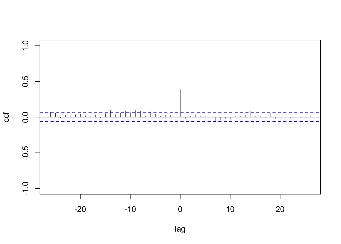
FIGURE 12.1: Sample CCF of the simulated Gaussian bivariate responses with diagonal \(\boldsymbol{W}\) and \(\boldsymbol{\Phi}\).
We show the formula for (12.3), which involves setting up indexes
id.V, id.b0.x1, and id.b0.x2.
Since R-INLA would fit a univariate Gaussian model by default, we must indicate
the requirement for a bivariate Gaussian model (i.e., \(q=2\)) by setting model="iid2d" in the formula chunk for . That is, the term
f(id.V, model = "iid2d", n = N) indicates that \(\boldsymbol V\) is assumed to be a non-diagonal covariance matrix for the bivariate responses, and follows an inverse Wishart prior.
In R-INLA, “iid2d” is represented internally as a single vector of length \(N=2n\), i.e.,
\((y_{1,1},\ldots, y_{1,n}, y_{2,1},\ldots, y_{2,n})\);
\(N\) is a required argument in the functional form for .
Since R-INLA only allows us to specify up to \(q=5\), the maximum allowed value of \(N\) is \(N=5n\), and we can correspondingly set up
model = “iid5d”. For more details, refer to inla.doc("iid").
The terms f(id.b0.x1, model = "ar1") and
f(id.b0.x2, model = "ar1") indicate how to fit independent AR(1) models to each of the state variables, which are independent because we assumed both
\(\boldsymbol \Phi\) and \(\boldsymbol W\) to be diagonal matrices.
We assume a Gaussian prior with high precision through the argument control.family (recall that control.family is used to define priors on the distribution of the response variable). We can verify from the results that the estimated values are close to the corresponding true values used in the simulation. The estimated level \(\alpha\) is close to zero (posterior mean is \(-0.059\) and posterior standard deviation is \(0.053\)), since we did not include a level in the simulated model.
m <- n - 1
N <- 2 * n
id.V <- 1:N
id.b0.x1 <- c(1:n, rep(NA, n))
id.b0.x2 <- c(rep(NA, n), 1:n)
biv.dat <- cbind.data.frame(y, id.b0.x1, id.b0.x2, id.V)
The formula and model fit are shown below.
formula.biv <-  y ~ 1 +
  f(id.V, model = "iid2d", n = N) +
  f(id.b0.x1, model = "ar1") +
  f(id.b0.x2, model = "ar1")
result.biv <- inla(
formula.biv,
family = c("gaussian"),
data = biv.dat,
control.inla = list(h = 1e-5, tolerance = 1e-3),
control.compute = list(dic = TRUE, config = TRUE),
control.predictor = list(compute = TRUE),
control.family = list(hyper = list(prec = list(
initial = 12, fixed = TRUE
)))
)
result.biv.summary <- summary(result.biv)format.inla.out(result.biv.summary$hyperpar[c(1,2)])
## name mean sd
## 1 Precision for id.V component 1 1.072 0.045
## 2 Precision for id.V component 2 0.686 0.027
## 3 Rho1:2 for id.V 0.635 0.015
## 4 Precision for id.b0.x1 0.758 0.097
## 5 Rho for id.b0.x1 0.767 0.016
## 6 Precision for id.b0.x2 4.287 0.980
## 7 Rho for id.b0.x2 0.587 0.060In the hyperparameter summary,
Precision for id.V (component 1) estimates the precision \(1/V_{11}\),
Precision for id.V (component 2) estimates the precision \(1/V_{22}\), and
Rho1:2 for id.V estimates the correlation \(R_{12}\). The estimates of the precisions for the state errors are given by Precision for id.b0.x1 and Precision for id.b0.x2, while the estimates for \(\phi_1\) and \(\phi_2\) are given by
Rho for id.b0.x1 and Rho for id.b0.x2.
12.2.3 Example: Ridesourcing data in NYC for a single taxi zone
We reconsider the ridesourcing data in NYC that we discussed in Chapter 6, where we treated scaled weekly TNC usage as a response variable and scaled Subway and Taxi usage as predictors, along with other time and location varying predictors. We now illustrate the multivariate DLM fit by treating scaled TNC and Taxi usage as a \(q=2\)-dimensional response vector and fit the model shown in (12.1) and (12.2) to data from a single taxi zone, i.e., Brooklyn Heights. The CCF plot for TNC usage and Taxi usage in Figure 12.2 shows significant negative correlation up to nearly \(20\) lags, with some evidence of nonstationary behavior.
ride.brooklyn <-
  read.csv("ride.brooklyn.csv",
           header = TRUE,
           stringsAsFactors = FALSE)
n <- n_distinct(ride.brooklyn$date)
n.hold <- 5
n.train <- n - n.hold
train.df <- ride.brooklyn[1:n.train, ]
test.df <- tail(ride.brooklyn, n.hold)
We construct a vectorized form of the bivariate response time series. \(N = 2n\) represents the length of the \(2\)-dimensional time series (i.e., \(q=2\)) stacked one below the other, and the response vector \(\boldsymbol y\) is the stacked time series consisting of scaled TNC and Taxi usage.
N <- 2 * n
y <-
  c(c(train.df$tnc, rep(NA, n.hold)), c(train.df$taxi, rep(NA, n.hold)))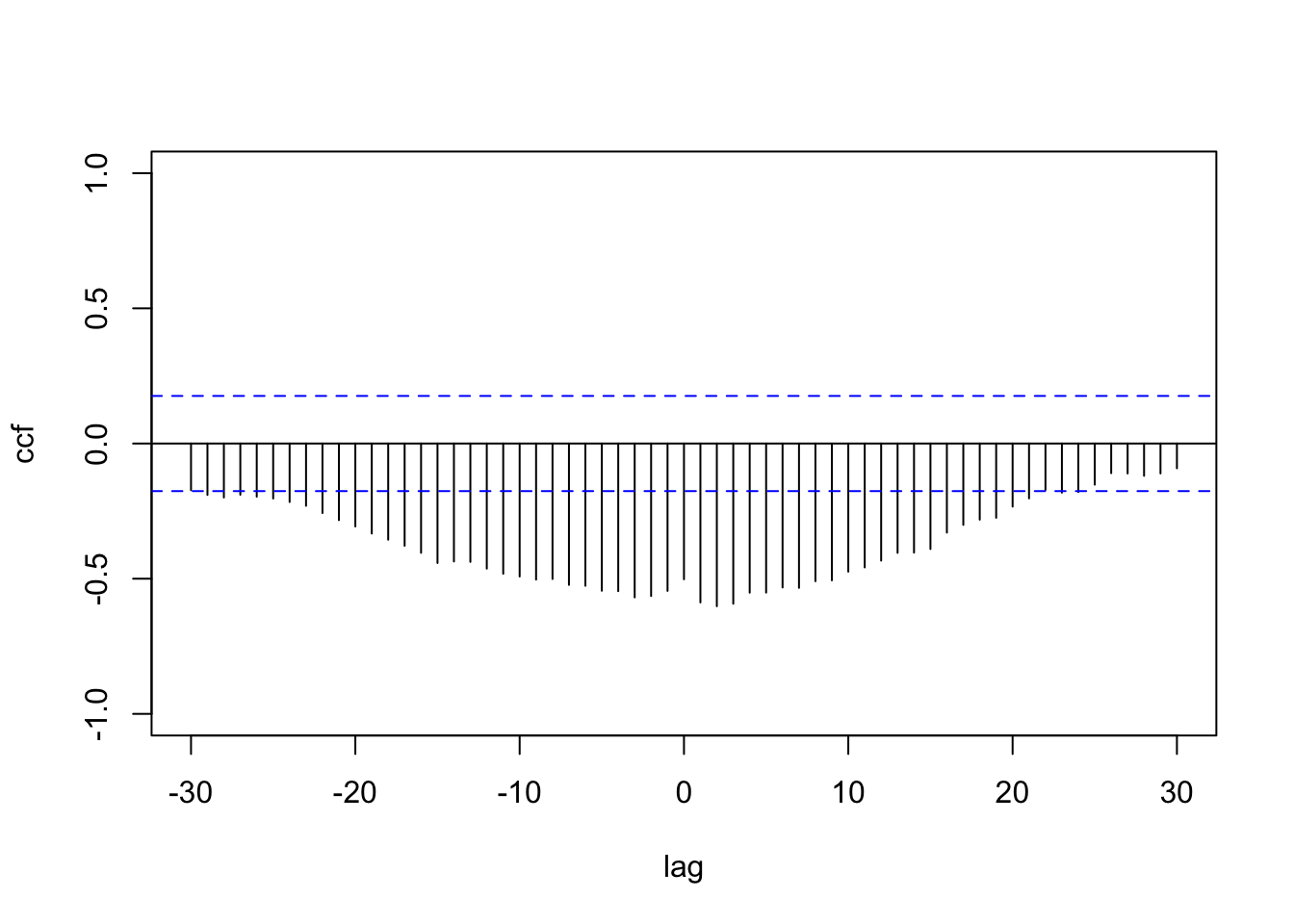
FIGURE 12.2: Sample CCF plot of TNC usage and Taxi usage.
We include Subway usage, holiday, and precipitation (these were described in Chapter 6) as exogenous variables with fixed effects (similar to the best fitting models in Chapter 6). Since \(q=2\), we construct two new variables for each predictor, one for each response. For example, to understand the impact of subway on TNC and Taxi usage, the new set of predictors is subway.tnc and subway.taxi. In subway.tnc, the last \(n\) values are NA’s since the last \(n\) values in \(\boldsymbol y\) correspond to data for scaled Taxi usage. Likewise, the first \(n\) values of subway.taxi are set as NA. In a similar fashion, we create indexes for the level, holidays, and precipitation.
alpha.tnc <- c(rep(1,n), rep(NA,n))
alpha.taxi <- c(rep(NA,n), rep(1,n))
subway.tnc <- c(ride.brooklyn$subway, rep(NA, n))
subway.taxi <- c(rep(NA, n), ride.brooklyn$subway)
holidays.tnc <- c(ride.brooklyn$holidays, rep(NA, n))
holidays.taxi <- c(rep(NA, n), ride.brooklyn$holidays)
precip.tnc <- c(ride.brooklyn$precip, rep(NA, n))
precip.taxi <- c(rep(NA, n), ride.brooklyn$precip)
t.index <- 1:N
b0.tnc <- c(1:n, rep(NA, n))
b0.taxi <- c(rep(NA, n), 1:n)
We then create a data frame as:
ride.mvn.data <- cbind.data.frame(y, alpha.tnc, alpha.taxi,
                                  subway.tnc, subway.taxi,
                                  holidays.tnc, holidays.taxi,
                                  precip.tnc, precip.taxi,
                                  b0.tnc, b0.taxi,
                                  t.index)
We fit a model to \(\boldsymbol y_t\) (consisting of time series of TNC and Taxi usage) as a function of a dynamic trend \(\boldsymbol{\beta}_{t,0}\) and static effects due to Subway usage (\(Z_{t,1}\)), holidays (\(Z_{t,2}\)), and precipitation (\(Z_{t,3}\)). The observation equations are
\[\begin{align} Y_{1,t} = \alpha_1 + \beta_{1,t,0} + \beta_{1,1} Z_{t,1} + \beta_{1,2} Z_{t,2} + \beta_{1,3} Z_{t,3} + v_{1,t}, \notag \\ Y_{2,t} = \alpha_2 + \beta_{2,t,0} + \beta_{2,1} Z_{t,1} + \beta_{2,2} Z_{t,2} + \beta_{2,3} Z_{t,3} + v_{2,t}, \tag{12.4} \end{align}\] where the observation error vector \(\boldsymbol{v}_t \sim N(\boldsymbol 0, \boldsymbol V)\) with \(\boldsymbol V\) being a \(2 \times 2\) p.d. covariance matrix. The state equation corresponding to the latent vector \(\boldsymbol{\beta}_{t,0} = (\beta_{1,t,0}, \beta_{2,t,0})'\) is
\[\begin{align} \boldsymbol{\beta}_{t,0} = \boldsymbol{\Phi} \boldsymbol{\beta}_{t-1,0} + \boldsymbol w_t, \tag{12.5} \end{align}\] where \(\boldsymbol w_t \sim N(\boldsymbol 0, \boldsymbol W)\), and \(\boldsymbol W\) and \(\boldsymbol{\Phi}\) are diagonal. This corresponds to \(q=2\) independent AR(1) processes.
We indicate the bivariate Gaussian assumption on \(\boldsymbol V\) by setting model="iid2d" in the formula chunk for t.index.
We also assume a Gaussian prior with high precision through the argument control.family, which is necessary in R-INLA for fitting MV models.
formula.ride.mvn.model1 <-  y ~ -1 + alpha.tnc + alpha.taxi +
   subway.tnc + subway.taxi +
   holidays.tnc + holidays.taxi +
   precip.tnc + precip.taxi +
  f(t.index, model="iid2d", n=N) +
  f(b0.tnc,model="ar1") +
  f(b0.taxi,model="ar1")
ride.mvn.model1 <-
inla(
formula.ride.mvn.model1,
family = c("gaussian"),
data = ride.mvn.data,
control.compute = list(dic = TRUE,
config = TRUE),
control.predictor = list(compute = TRUE),
control.family =
list(hyper = list(prec = list(
initial = 10,
fixed = TRUE
))),
)
format.inla.out(ride.mvn.model1$summary.hyperpar[c(1,2)])
## name mean sd
## 1 Precision for t.index component 1 91.189 12.230
## 2 Precision for t.index component 2 83.944 11.334
## 3 Rho1:2 for t.index 0.088 0.093
## 4 Precision for b0.tnc 12.851 7.412
## 5 Rho for b0.tnc 0.994 0.003
## 6 Precision for b0.taxi 265.084 166.161
## 7 Rho for b0.taxi 0.955 0.030In the hyperparameter summary,
Precision for t.index (component 1) estimates the precision for TNC, \(1/V_{11}\),
Precision for t.index (component 2) estimates the precision for Taxi, \(1/V_{22}\), and Rho1:2 for t.index estimates the correlation between \(R_{12}\), which is not significant.
The estimates of the precisions for the state errors are given by Precision for b0.tnc and Precision for b0.taxi, while the estimates for \(\phi_1\) and \(\phi_2\) are given by
Rho for b0.tnc and Rho for b0.taxi.
Fitted values and forecasts in multivariate DLMs
The steps used to obtain fitted values in the multivariate framework are different from what we presented in Chapter 3 for the univariate case. We can adopt two different coding approaches to obtain fitted values in the multivariate case. The first approach uses inla.posterior.samples() to construct samples of the predictive distributions of the responses. The second approach uses inla.make.lincomb() and then fits the model.
Approach 1.
Recall that inla.posterior.samples() provides \(M\) (a user chosen number; here, \(M=1000\)) posterior samples for the model parameters and hyperparameters. For each \(m=1,\ldots,M\), we can use these posterior values to simulate fitted responses from the model structure in (12.4) and (12.5). For each of the \(q=2\) components, the sample average of these \(M\) fitted response values for each time \(t\) constitutes a fitted time series, which can then be plotted against the observed TNC and Taxi usages, as shown in Figure 12.3.
post.sample <-
  inla.posterior.sample(1000, ride.mvn.model1)
We source the function below which computes the fitted values based on the model formula given the posterior samples.
fit.post.sample <- function(x) {
  sigma2.v1 <- 1 / x$hyperpar[1]
  sigma2.v2 <- 1 / x$hyperpar[2]
  rho.v1v2 <- x$hyperpar[3]
  cov.v1v2 <- rho.v1v2 * sqrt(sigma2.v1) * sqrt(sigma2.v2)
  sigma.v <-
    matrix(c(sigma2.v1, cov.v1v2, cov.v1v2, sigma2.v2), nrow = 2)
  V <- rmvnorm(n, mean = c(0, 0), sigma = sigma.v)
  V1 <- V[, 1]
  V2 <- V[, 2]
  fit.tnc <- x$latent[grep("alpha.tnc", rownames(x$latent))] +
    x$latent[grep("b0.tnc", rownames(x$latent))] +
    x$latent[grep("subway.tnc", rownames(x$latent))] *
    ride.brooklyn$subway +
    x$latent[grep("holidays.tnc", rownames(x$latent))] *
    ride.brooklyn$holidays +
    x$latent[grep("precip.tnc", rownames(x$latent))] *
    ride.brooklyn$precip +
    V1
  fit.taxi <- x$latent[grep("alpha.taxi", rownames(x$latent))] +
    x$latent[grep("b0.taxi", rownames(x$latent))] +
    x$latent[grep("subway.taxi", rownames(x$latent))] *
    ride.brooklyn$subway +
    x$latent[grep("holidays.taxi", rownames(x$latent))] *
    ride.brooklyn$holidays +
    x$latent[grep("precip.taxi", rownames(x$latent))] *
    ride.brooklyn$precip +
    V2
  return(list(fit.tnc = fit.tnc, fit.taxi = fit.taxi))
}
The fitted values for TNC usage and Taxi usage can be obtained for each set of generated parameters, and the averages over \(M=1000\) samples are saved as tnc.fit and taxi.fit.
fits <- post.sample %>%
  lapply(function(x)
    fit.post.sample(x))
tnc.fit <- fits %>%
  sapply(function(x)
    x$fit.tnc) %>%
  rowMeans()
taxi.fit <- fits %>%
  sapply(function(x)
    x$fit.taxi) %>%
  rowMeans()
Figure 12.3 shows the fitted versus observed values for TNC usage (top plot) and Taxi usage (bottom plot). The model fit is close for most of the training period. While the forecasts for Taxi usage in the test period are accurate, the model seems to under predict actual TNC usage which appears to have an upswing for those time periods.
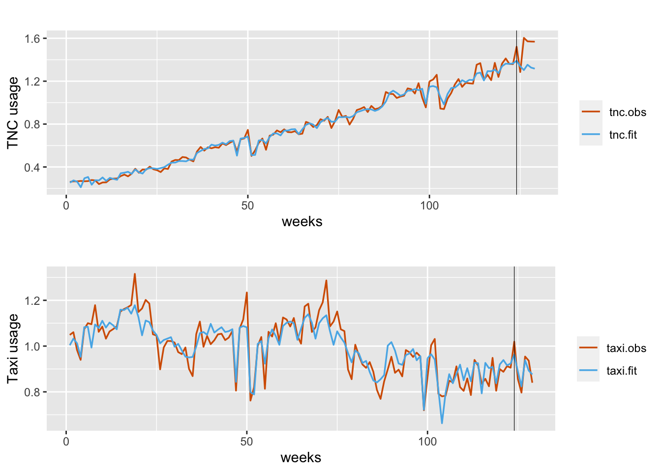
FIGURE 12.3: Observed (red) versus fitted (blue) TNC (top panel) and Taxi usage (bottom panel). Fits obtained using inla.posterior.sample(). The black vertical line divides the data into training and test portions.
Approach 2.
We set up and use linear combinations of the latent random field (for details, see Martins et al. (2013)). Specifically, for model fitting and prediction, we use inla.make.lincomb(), which creates a list for every \(t\) with idx and weight, where weight is the value of the predictor corresponding to the time index idx. The setup for TNC is shown below.
lc1 <- c()
tnc.dat.lc <- ride.brooklyn %>%
  select(subway, holidays:precip)
for(i in 1:n){
  idx0 <- idx1 <- idx2 <- idx3 <-  rep(0,n)
  idx0[i] <-  1
  idx1[i] <- tnc.dat.lc[i,1]
  idx2[i] <- tnc.dat.lc[i,2]
  idx3[i] <- tnc.dat.lc[i,3]
  lcc <-  inla.make.lincomb(alpha.tnc=1, b0.tnc = idx0, subway.tnc=idx1[i],
                            holidays.tnc = idx2[i], precip.tnc = idx3[i])
  for (k in 1:length(lcc[[1]])) {
    if(length(lcc[[1]][[k]][[1]]$weight)==0){
      lcc[[1]][[k]][[1]]$idx <- i
      lcc[[1]][[k]][[1]]$weight <- 0
    }
  }
  names(lcc) <-  paste0("tnc", i)
  lc1 <-  c(lc1, lcc)
}
The setup for Taxi usage is similar.
lc2 <- c()
taxi.dat.lc <- ride.brooklyn %>%
  select(subway, holidays:precip)
for (i in 1:n) {
  idx0 <- idx1 <- idx2 <- idx3 <-  rep(0, n)
  idx0[i] <-  1
  idx1[i] <- taxi.dat.lc[i, 1]
  idx2[i] <- taxi.dat.lc[i, 2]
  idx3[i] <- taxi.dat.lc[i, 3]
  lcc <-
    inla.make.lincomb(
      alpha.taxi = 1,
      b0.taxi = idx0,
      subway.taxi = idx1[i],
      holidays.taxi = idx2[i],
      precip.taxi = idx3[i]
    )
  for (k in 1:length(lcc[[1]])) {
    if (length(lcc[[1]][[k]][[1]]$weight) == 0) {
      lcc[[1]][[k]][[1]]$idx <- i
      lcc[[1]][[k]][[1]]$weight <- 0
    }
  }
  names(lcc) <-  paste0("taxi", i)
  lc2 <-  c(lc2, lcc)
}
We then combine the linear combinations into lc as follows.
lc <- c(lc1, lc2)The list lcc contains the index number (time), the values for fixed predictors, and latent intercepts \(\beta_{1,t,0}\) and \(\beta_{2,t,0}\). For example, the components of lc1[[5]] will show values of the predictors at time \(t = 5\):
lc1[[5]]We include the list of linear combinations created in our model fitting using the argument lincomb = lc in the inla() call. This enables us to obtain posterior marginals of the linear combinations, as shown below. Also note that the model output will not include a “Precision for Gaussian observation” term, due to our assumption of a large and fixed precision.
ride.mvn.model1 <-
  inla(
    formula.ride.mvn.model1,
    family = c("gaussian"),
    data = ride.mvn.data,
    control.compute = list(dic = TRUE, config = TRUE),
    control.predictor = list(compute = TRUE),
    control.family =
      list(hyper = list(prec = list(
        initial = 10,
        fixed = TRUE
      ))),
    lincomb = lc
  )
format.inla.out(ride.mvn.model1$summary.hyperpar[c(1, 2)])
##   name                              mean    sd
## 1 Precision for t.index component 1  91.193  12.230
## 2 Precision for t.index component 2  83.940  11.335
## 3 Rho1:2 for t.index                  0.088   0.093
## 4 Precision for b0.tnc               12.677   7.328
## 5 Rho for b0.tnc                      0.995   0.003
## 6 Precision for b0.taxi             263.002 163.498
## 7 Rho for b0.taxi                     0.956   0.029
Plots of fitted versus observed usage for TNC and Taxi usage are shown in Figure 12.4.
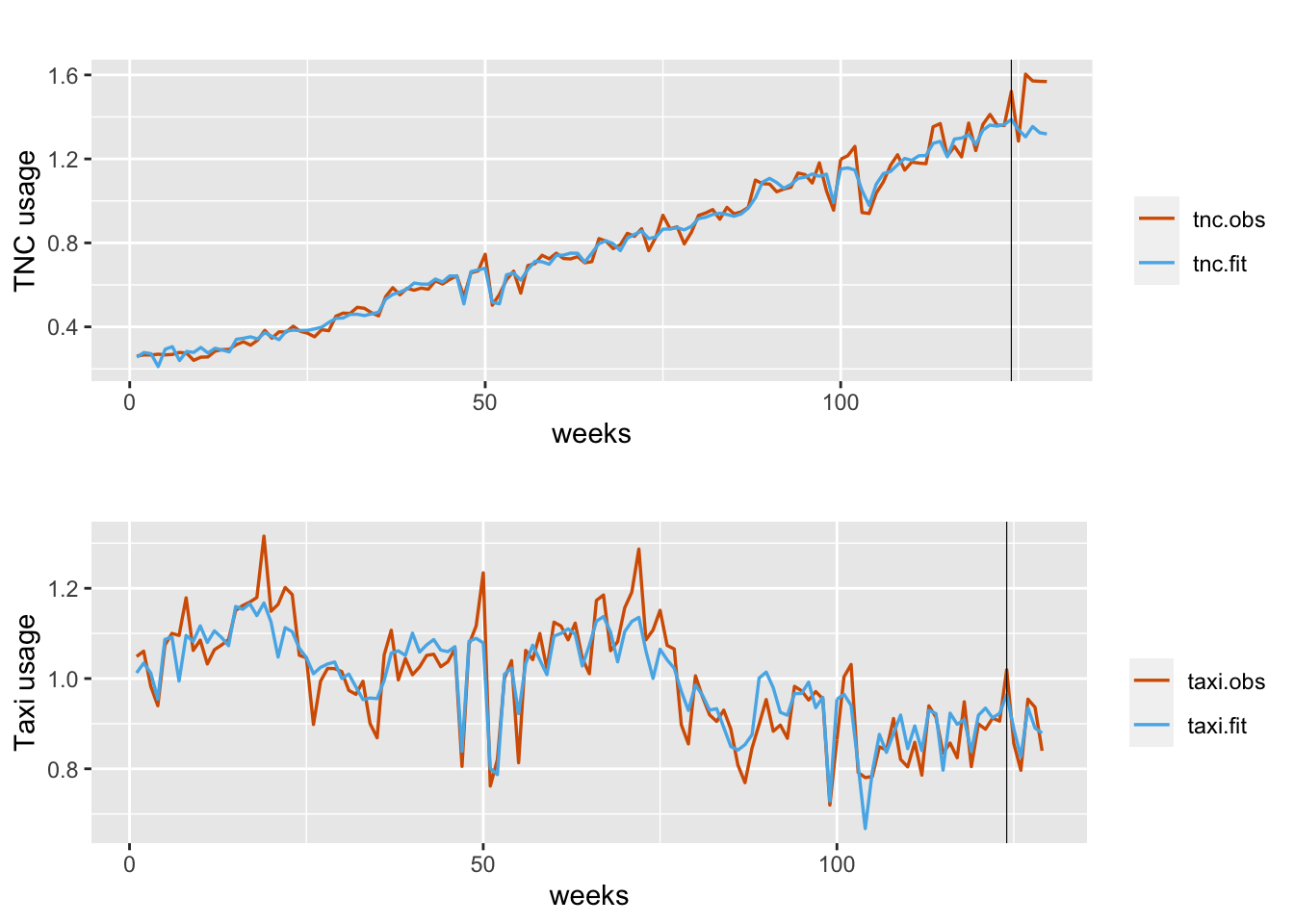
FIGURE 12.4: Observed (red) versus fitted (blue) TNC usage (top panel) and Taxi usage (bottom panel). Fits obtained using inla.make.lincomb(). The black vertical line divides the data into training and test portions.
We end this section with a few useful remarks.
Remark 1. If we wish to modify the inverse Wishart prior specification, we can use the code given below.
formula.ride.mvn.model1 <-  y ~ -1 +
  f(t.index,
    model = "iid2d",
    n = N,
    hyper = list(theta1 = list(param = c(4, 0.01, 0.01, 0)))) + ...
We see that differences due to the different prior specifications are minimal for large \(n\).
Remark 2. If we wish to include the effects of the exogenous predictors as dynamic random effects, rather than fixed effects as shown above, the following code is useful. Setting up the linear combinations is similar to the fixed effects case; the only change is that we replace the name of the predictor by its index. For example, we replace subway.tnc (which contains data on Subway usage for the first \(n\) rows and NA’s for the next \(n\) rows) with id.sub.tnc (which is a vector with \(1:n\) followed by \(n\) NA’s). The variables subway.taxi and id.sub.taxi will have the Subway usage data or \(1:n\) switched with the NA’s.
t.index <- 1:N
alpha.tnc <- c(rep(1,n), rep(NA,n))
alpha.taxi <- c(rep(NA,n), rep(1,n))
b0.tnc <- id.sub.tnc <-
  id.holidays.tnc <- id.precip.tnc <- c(1:n, rep(NA, n))
b0.taxi <- id.sub.taxi <- id.events.taxi <-
  id.holidays.taxi <- id.precip.taxi <- c(rep(NA, n), 1:n)
ride.mvn.data <- cbind.data.frame(
  y,alpha.tnc,alpha.taxi,subway.tnc,subway.taxi,holidays.tnc,
  holidays.taxi,precip.tnc,precip.taxi,
  b0.tnc,b0.taxi,id.sub.tnc,
  id.sub.taxi,id.holidays.tnc,id.holidays.taxi,
  id.precip.tnc,id.precip.taxi,t.index
)
In the formula, we then replace the fixed effects by suitable random effect specifications as shown below.
formula.ride.mvn.model1 <-  y ~ -1 + alpha.tnc + alpha.taxi +
  f(t.index, model = "iid2d", n = N) +
  f(b0.tnc, model = "ar1", constr = FALSE) +
  f(b0.taxi, model = "ar1", constr = FALSE) +
  f(id.sub.tnc, subway.tnc, model = "ar1", constr = FALSE) +
  f(id.sub.taxi, subway.taxi, model = "ar1", constr = FALSE) +
  f(id.holidays.tnc,
    holidays.tnc,
    model = "ar1",
    constr = FALSE) +
  f(id.holidays.taxi,
    holidays.taxi,
    model = "ar1",
    constr = FALSE) +
  f(id.precip.tnc,
    precip.tnc,
    model = "ar1",
    constr = FALSE) +
  f(id.precip.taxi,
    precip.taxi,
    model = "ar1",
    constr = FALSE)
Corresponding linear combinations can then be similarly constructed, as shown below for TNC usage. The construction for Taxi usage will be similar.
lc1 <- c()
tnc.dat.lc <- ride.brooklyn %>%
  select(subway, holidays:precip)
for(i in 1:n){
  idx0 <- idx1 <- idx2 <- idx3 <-  rep(0,n)
  idx0[i] <-  1
  idx1[i] <- tnc.dat.lc[i,1]
  idx2[i] <- tnc.dat.lc[i,2]
  idx3[i] <- tnc.dat.lc[i,3]
  lcc <-  inla.make.lincomb(b0.tnc=idx0, id.sub.tnc=idx1,
                            id.holidays.tnc = idx2, id.precip.tnc = idx3)
  for (k in 1:length(lcc[[1]])) {
    if(length(lcc[[1]][[k]][[1]]$weight)==0){
      lcc[[1]][[k]][[1]]$idx <- i
      lcc[[1]][[k]][[1]]$weight <- 0
    }
  }
  names(lcc) <-  paste0("tnc", i)
  lc1 <-  c(lc1, lcc)
}
Remark 3.
Note that the current version of the function inla.make.lincomb() gives an error when a predictor value is \(0\) (for example, in holidays or precipitation), the reason being that a weight=0 corresponding to this \(0\) value has now been coded as NA in R-INLA.9 To circumvent this, we include a workaround by the following lines of code which replace weight = NA by weight=0:
for (k in 1:length(lcc[[1]])) {
    if(length(lcc[[1]][[k]][[1]]$weight)==0){
      lcc[[1]][[k]][[1]]$idx <- i
      lcc[[1]][[k]][[1]]$weight <- 0
    }
  }
12.3 Model with equicorrelated \(\boldsymbol{w}_t\) and diagonal \(\boldsymbol \Phi\)
Let \(\boldsymbol \Phi\) be diagonal, while \(Cov(\boldsymbol{w}_t) = \boldsymbol W = \sigma^2_w [(1-\rho_w)\boldsymbol I + \rho_w \boldsymbol J]\), where \(\boldsymbol I\) is the \(p \times p\) identity matrix and \(\boldsymbol J\) is the \(p \times p\) matrix whose entries are all 1. That is, components of the state error vector \(\boldsymbol w_t\) are correlated, such that the correlation between any pair of components is the same \(|\rho_w| < 1\) (intra-class correlation or equi-correlation structure). We model simulated trivariate Gaussian time series with this structure using the group option.
12.3.1 Example: Simulated trivariate series
We simulate a trivariate series \(\boldsymbol{y}_t\). The observation error covariance \(\boldsymbol{V}\) is set up below.
V.11 <- 1.0
V.22 <- 1.0
V.33 <- 1.0
R.12 <- 0.7
R.13 <- 0.4
R.23 <- 0.25
V.12 <- R.12 * sqrt(V.11) * sqrt(V.22)
V.13 <- R.13 * sqrt(V.11) * sqrt(V.33)
V.23 <- R.23 * sqrt(V.22) * sqrt(V.33)
V <- matrix(c(V.11, V.12, V.13, V.12, V.22, V.23,
              V.13, V.23, V.33), nrow = 3)
The state error covariance \(\boldsymbol{W}\) has the equicorrelation structure.
sig2.w <- 0.1
rho.w <- 0.75
W.11 <- sig2.w
W.22 <- sig2.w
W.33 <- sig2.w
W.12 <- sig2.w*rho.w
W.13 <- sig2.w*rho.w
W.23 <- sig2.w*rho.w
W <- matrix(c(W.11, W.12, W.13, W.12, W.22, W.23,
              W.13, W.23, W.33), nrow = 3)
We assume that each AR(1) coefficient has the same value \(\phi\). We then set up the
arrays \(\boldsymbol{I}_3\) and diag\((\phi_1, \phi_2, \phi_3)\) to be fed as parameters in the marima.sim() function in the R package . Note that the \(\phi\) value in this package corresponds to the AR polynomial \((1+ \phi B)\) and not \((1 - \phi B)\), which is the usual convention.
phi.1 <- -0.5
phi.2 <- -0.5
phi.3 <- -0.5
# Set up Phi as be a 3-dim array
Phi <- array(0, dim = c(3, 3, 2))
Phi[1,1,1] <- 1.0
Phi[2,2,1] <- 1.0
Phi[3,3,1] <- 1.0
Phi[1,1,2] <- phi.1
Phi[2,2,2] <- phi.2
Phi[3,3,2] <- phi.3
We simulate the states from VAR(1) processes using the package.
n <- n.sim <- 1000
q <- 3
n.start <- 0
avg <- rep(0, 3)
X <-
  marima.sim(
    3,
    ar.model = Phi,
    ar.dif = NULL,
    ma.model = NULL,
    averages = rep(0, 3),
    resid.cov = W,
    seed = 1234,
    nstart = n.start,
    nsim = n.sim
  )
x1 <- X[, 1]
x2 <- X[, 2]
x3 <- X[, 3]
Figure 12.5 shows the ACF plots for the three state vector components, with \(\phi = -0.5\).
par(mfrow=c(1,3))
acf(x1, main ="", sub="ACF of x1")
acf(x2, main ="", sub="ACF of x2")
acf(x3, main ="", sub="ACF of x3")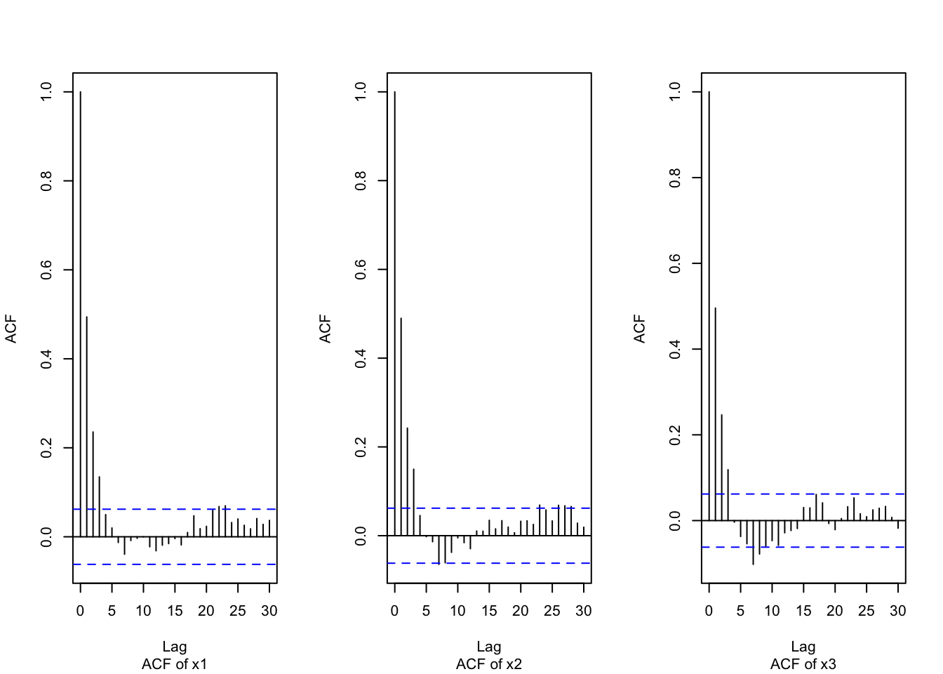
FIGURE 12.5: ACF’s of the trivariate state series (\(\phi = -0.5\)).
We next simulate observation errors from a \(N_3(\boldsymbol{0}, \boldsymbol{V})\) distribution, and add these to the states to get the response time series \(\boldsymbol{y}_t\). Figure 12.6 shows the CCF of \(\boldsymbol{x}_t\) (top row), and the CCF of \(\boldsymbol{y}_t\) (bottom row).
# Generate observation errors
set.seed(123457)
err.v <- rmvnorm(n.sim, mean = c(0, 0, 0), sigma = V)
err.v1 <- err.v[, 1]
err.v2 <- err.v[, 2]
err.v3 <- err.v[, 3]
# Add observation errors to states to get responses
y1 <- x1 + err.v1
y2 <- x2 + err.v2
y3 <- x3 + err.v3
y <- c(y1, y2, y3)par(mfrow=c(2,3))
ccf(x1, x2, ylab = "CCF", main ="", sub="CCF of (x1,x2)")
ccf(x1, x3, ylab = "CCF", main ="", sub="CCF of (x1,x3)")
ccf(x2, x3, ylab = "CCF", main ="", sub="CCF of (x2,x3)")
ccf(y1,y2, main="", sub="CCF of (y1,y2)")
ccf(y1,y3, main="", sub="CCF of (y1,y3)")
ccf(y2,y3, main="", sub="CCF of (y2,y3)")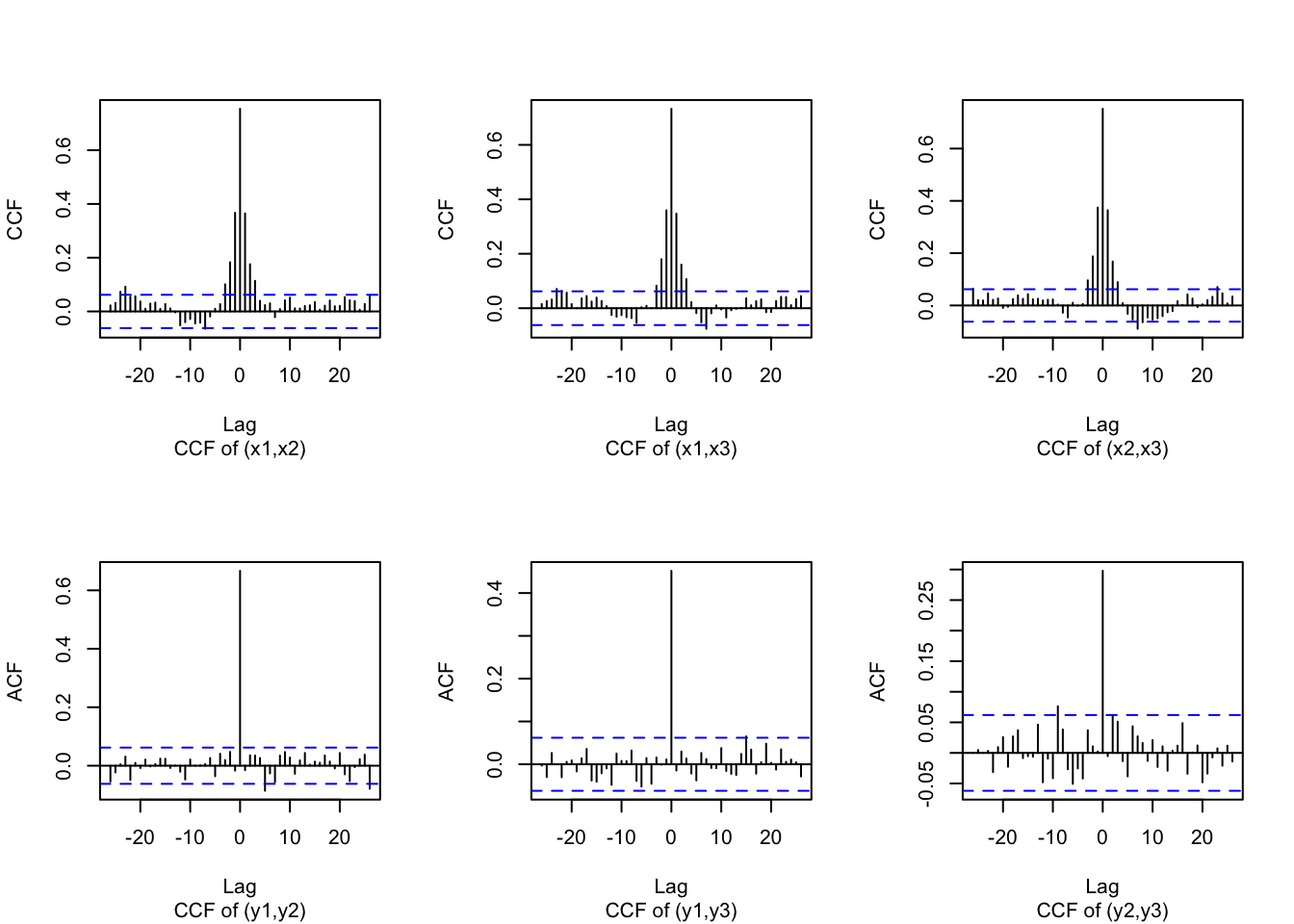
FIGURE 12.6: CCF’s of the trivariate state and response time series.
The formula and model fit follow. Note that id.b0.g <- rep(1:3, each = n) allows us to incorporate a grouping that reflects the equicorrelated state errors and the same \(\phi\) in the the diagonal of \(\boldsymbol{\Phi}\) in the
VAR\((1)\) model for the state vector (dynamic intercept).
This is used in the
line f(id.b0, model="ar1", constr = FALSE, group = id.b0.g). As in Section 12.2, f(id.V, model="iid3d", n=N) allows a trivariate inverse Wishart specification for \(\boldsymbol V\).
m <- n-1
N <- 3*n
id.V <- 1:N
id.b0 <- c(1:n, 1:n, 1:n)
id.b0.g <- rep(1:3, each = n)
triv.dat <- cbind.data.frame(y, id.b0, id.b0.g, id.V)
formula.triv <-  y ~ 1 +
  f(id.V, model="iid3d", n=N) +
  f(id.b0, model="ar1", constr = FALSE, group = id.b0.g)
result.triv <-
inla(
formula.triv,
family = c("gaussian"),
data = triv.dat,
control.inla = list(h = 1e-5, tolerance = 1e-3),
control.compute = list(dic = TRUE, config = TRUE),
control.predictor = list(compute = TRUE),
control.family = list(hyper = list(prec = list(
initial = 12, fixed = TRUE
)))
)
result.triv.summary <- summary(result.triv)format.inla.out(result.triv.summary$hyperpar[c(1,2)])
## name mean sd
## 1 Precision for id.V component 1 0.958 2.700e-02
## 2 Precision for id.V component 2 0.951 2.700e-02
## 3 Precision for id.V component 3 0.860 2.800e-02
## 4 Rho1:2 for id.V 0.668 1.300e-02
## 5 Rho1:3 for id.V 0.453 1.900e-02
## 6 Rho2:3 for id.V 0.299 2.000e-02
## 7 Precision for id.b0 1304.921 5.537e+16
## 8 Rho for id.b0 -0.520 2.180e-01
## 9 GroupRho for id.b0 0.869 6.600e-02The first three rows in the output provide posterior summaries for the precisions of the components of \(\boldsymbol{v}_t\), whose true values are \(1.0\).
The next three rows are posterior summaries of the correlations between the components of
\(\boldsymbol{v}_t\), whose true values are \(R_{12}=0.7, R_{13}=0.4\), and \(R_{23}=0.25\).
The value Rho for id.b0 estimates the common \(\phi\), with true value \(-0.5\).
The term GroupRho for id.b0 estimates the equicorrelation coefficient \(\rho_w\), whose true value is \(0.75\). We can recover \(\sigma^2_w\) by dividing Precision for id.b0 by \(1-\phi^2\).
Again, to obtain fitted values and predictions, we can either use inla.posterior.samples() or inla.make.lincomb() (see the detailed discussion in Section 12.2).
12.4 Fitting multivariate models using rgeneric
In vector time series modeling, we often need to fit models with a full (non-diagonal) \(\boldsymbol \Phi\) matrix, and/or an unstructured state error covariance matrix \(\boldsymbol{W}\).
To the best of our knowledge, no R-INLA template currently exists for fitting such a model. Instead, we implement this by using the rgeneric() function.
Gómez-Rubio (2020) used the rgeneric() function to fit a conditionally autoregressive (CAR) specification to latent spatial random effects, while Palmı́-Perales, Gómez-Rubio, and Martinez-Beneito (2021) discussed multivariate spatial models for lattice data. For more details, see the example discussed in vignette("rgeneric", package = INLA).
Here, we illustrate the use of the rgeneric() function for fitting a VAR(1) state equation (see Dutta, Ravishanker, and Basu (2022) for more details).
In using rgeneric(), the user directly computes the likelihood and priors that are required for the model specification of interest.
The function inla.rgeneric.define() defines the different latent effects, and takes as arguments functions such as graph(), Q(), etc., along with other arguments that are required to evaluate the different functions.
12.4.1 Example: Simulated bivariate VAR(1) series
We simulate bivariate time series from a model whose observation and state equations are given below:
\[\begin{align} \boldsymbol{y}_t & = \boldsymbol{x}_t + \boldsymbol{v}_t, \notag \\ \boldsymbol{x}_t & = \boldsymbol{\Phi}\boldsymbol{x}_{t-1} + \boldsymbol{w}_t, \tag{12.6} \end{align}\] where \(\boldsymbol{v}_t \sim N(\boldsymbol{0}, \boldsymbol{V})\) with \(\boldsymbol{V} = \begin{pmatrix} 1/\tau_{11} & R_{12}/\sqrt{\tau_{11}\tau_{22}} \\ R_{12}/\sqrt{\tau_{11}\tau_{22}} & 1/\tau_{22} \end{pmatrix},\) \(\tau_{ii}\) is the marginal precision of the \(i\)th component of \(\boldsymbol{V}\), \(i=1,2\), and \(R_{12}\) is the correlation between the two components of \(\boldsymbol{V}\). Here, \(\boldsymbol{\Phi} = \begin{pmatrix}\phi_{11} & \phi_{12} \\\phi_{21} & \phi_{22} \end{pmatrix}\), and \(\boldsymbol{W} = {\rm diag}(1/\tau_{w1}, 1/\tau_{w2})\), \(\tau_{wi}\) being the marginal precision of the \(i^{th}\) component of \(\boldsymbol{w}_t\), \(i=1,2\). Let \(\boldsymbol{\Theta} = (\phi_{11},\phi_{12},\phi_{21},\phi_{22},\tau_{w1},\tau_{w2},\tau_{11},\tau_{22},R_{12})'\). The data is simulated using the code below and these true parameter values:
\(\boldsymbol{\Phi} = \begin{pmatrix}0.7 & 0.1 \\0.3 & 0.2 \end{pmatrix}\), \(\boldsymbol{V} = \begin{pmatrix}1/2 & 0.55/\sqrt{2\times 3} \\0.55/\sqrt{2\times 3} & 1/3 \end{pmatrix}\), and \(\boldsymbol{W} = \begin{pmatrix}1/2 & 0 \\0 & 1/2 \end{pmatrix}\).
set.seed(123456)
p <- 1
k <- 2
n <- 300
phi.mat <- matrix(c(0.7,0.3,0.1,0.2),nrow=2,byrow=TRUE)
# Construct the W matrix
init.val <- matrix(c(0, 0))
rho.w1w2 = 0
sigma2.w1 <- 1 / 2
sigma2.w2 <- 1 / 2
cov.w1w2 <- rho.w1w2 * sqrt(sigma2.w1 * sigma2.w2)
sigma.mat.w <-
  matrix(c(sigma2.w1, cov.w1w2, cov.w1w2, sigma2.w2),
         nrow = 2,
         byrow = T)
sample.list <- list()
sample.list[[1]] <- init.val
for (i in 2:n) {
sample.list[[i]] <-
phi.mat %*% sample.list[[i - 1]] + matrix(MASS::mvrnorm(
n = 1,
mu = c(0, 0)
,
Sigma = sigma.mat.w
))
}
simulated_var <- do.call(cbind, sample.list)
var.ts <- t(simulated_var)
colnames(var.ts) <- c("y1", "y2")
x.t <- vec(var.ts)We set up the true \(\boldsymbol{V}\) matrix and simulate \(\boldsymbol{y}_t\).
rho.v1v2 = 0.55
sigma2.v1 <- 1 / 2
sigma2.v2 <- 1 / 3
cov.v1v2 <- rho.v1v2 * sqrt(sigma2.v1 * sigma2.v2)
sigma.mat.v <-
  matrix(c(sigma2.v1, cov.v1v2, cov.v1v2, sigma2.v2),
         nrow = 2,
         byrow = T)
v.t <- vec(mvrnorm(n, mu = c(0, 0), Sigma = sigma.mat.v))
y.t <- x.t + v.t
We next set up indexes and the data frame.
inla.dat <- data.frame(y = y.t, iid2d.id = 1:length(y.t))
odd.id <- seq(1, nrow(inla.dat), by = 2)
even.id <- seq(2, nrow(inla.dat), by = 2)
var.id <- c(odd.id, even.id)
inla.dat$var.id <- var.id
We source the function inla.rgeneric.VAR_1(), which is included in the list of custom functions, and is shown in Chapter 14.
Brief descriptions of the functions used within inla.rgeneric.VAR_1() are given below. For details on the formulas, see Lütkepohl (2013), Rue and Held (2005), and Chapter 12 – Appendix.
graph()defines which entries of a user defined precision matrixQ()are non-zero:
graph = function() {
      return (inla.as.sparse(Q()))
}- The precision matrix \(\boldsymbol{Q}(\boldsymbol{\theta})\) is computed in sparse form by using the function
Q(), withparamdenoting the model parameters:
Q <- function() {
  param <- interpret.theta()
  phi.mat <- matrix(param$phi.vec, nrow = k)
  sigma.w.inv <- param$PREC
  A <- t(phi.mat) %*% sigma.w.inv %*% phi.mat
  B <- -t(phi.mat) %*% sigma.w.inv
  C <- sigma.w.inv
  # Construct mid-block
  zero.mat <- matrix(0, nrow = 2, ncol = 2 * n)
  # Define the matrix block
  mat <- cbind(t(B), A + C, B)
  # Initializing column id and matrix list
  col.id <- list()
  mat.list <- list()
  col.id[[1]] <- 1:(3 * k)
  mat.list[[1]] <- zero.mat
  mat.list[[1]][, col.id[[1]]] <- mat
  for (id in 2:(n - 2)) {
    start.id <- col.id[[id - 1]][1] + k
    end.d <-  start.id + (3 * k - 1)
    col.id[[id]] <- start.id:end.d
    mat.list[[id]] <- zero.mat
    mat.list[[id]][, col.id[[id]]] <- mat
  }
  mid.block <- do.call(rbind, mat.list)
  tau.val <- 0.1
  diffuse.prec <- tau.val * diag(1, k)
  # Construct first and last row blocks and then join with mid block
  first.row.block <-
    cbind(A + diffuse.prec, B, matrix(0, nrow = k, ncol = (k * n - k ^ 2)))
  last.row.block <- cbind(matrix(0, nrow = k, ncol = k * n - k ^ 2), t(B),C)
  toep.block.mat <-
    rbind(first.row.block, mid.block, last.row.block)
  # Changing to a sparse Matrix
  prec.mat <- Matrix(toep.block.mat, sparse = TRUE)
  return(prec.mat)
}- The function
mu()is a zero vector:
mu <- function() {
      return(numeric(0))
}- The function
initial()contains initial values of the parameter \(\Theta\) expressed inR-INLA’s internal scale:
initial = function() {
  phi.init <- c(0.1, 0.1, 0.1, 0.1)
  prec.init <- rep(1, k)
  init <- c(phi.init, prec.init)
  return (init)
}log.norm.constant()denotes the logarithm of the normalizing constant from a multivariate Gaussian distribution. If we assignnumeric(0),R-INLAwill compute this constant.
log.norm.const <- function() {
  Q <- Q()
  log.det.val <-
    Matrix::determinant(Q, logarithm = TRUE)$modulus
  val <- (-k * n / 2) * log(2 * pi) + 0.5 * log.det.val
  return (val)
}- The function
log.prior()specifies the priors for the original model parameters on the log scale. Note that althoughR-INLAworks with internal variables (see Chapter 3), the log prior is set on the original parameters, such as \(\tau_{11}, \tau_{22}, R_{12}\), etc. We also include a term for the logarithm of the Jacobian of the transformations from the original to the internal scale of the parameters. Specifically, we set up a normal prior for each of the elements of the \(\boldsymbol{\Phi}\) matrix, and log gamma priors for each of the precisions from the \(\boldsymbol{W}\) matrix.
log.prior <- function() {
  param <- interpret.theta()
  pars <- param$param
  k <- k
  total.par <- param$n.phi + param$n.prec
  # Normal prior for phi's
  theta.phi <- theta[1:param$n.phi]
  phi.prior <-
    sum(sapply(theta.phi, function(x)
      dnorm(
        x, mean = 0, sd = 1, log = TRUE
      )))
  theta.prec <-
    theta[(param$n.phi + 1):(param$n.phi + param$n.prec)]
  prec.prior <-
    sum(sapply(theta.prec, function(x)
      dgamma(
        x,
        shape = 1,
        scale = 1,
        log = TRUE
      )))
  prec.jacob <- sum(theta.prec)
  prior.val <- phi.prior + prec.prior + prec.jacob
  return (prior.val)
}
The different functions described above are then pulled into the inla.rgeneric.VAR_1() function.
The complete set of functions can be accessed from inla.rgeneric.VAR_1() in Section 14.3.1. We can also obtain it from
the GitHub link for the book.
If we use R version 4.0 or higher, R-INLA gives a small fix that we must add to our code. These are also shown in the code below.
inla.rgeneric.VAR_1 <-
  function(cmd = c("graph",
                   "Q",
                   "mu",
                   "initial",
                   "log.norm.const",
                   "log.prior",
                   "quit"),
           theta = NULL)
  {
    envir = parent.env(environment())
    graph = function() {
      ...
    }
    Q = function() {
      ...
    }
    mu = function() {
      ...
    }
    log.norm.const = function() {
      ...
    }
    log.prior = function() {
      ...
    }
    initial = function() {
      ...
    }
    quit = function() {
      ...
    }
# Fix for R version higher than 4.0
    if (as.integer(R.version$major) > 3) {
      if (!length(theta))
        theta <- initial()
    } else {
      if (is.null(theta)) {
        theta <- initial()
      }
    }
    val <- do.call(match.arg(cmd), args = list())
    return (val)
The function interpret.theta() enables us to obtain the list of original parameters, along with the items used for the setup, such as the number of elements in \(\boldsymbol{\Phi}\), number of precision parameters in
\(\boldsymbol{W}\), etc.
interpret.theta <- function(theta) {
  n.phi <- k * k * p
  n.prec <- k
  n.tot <- n.phi + n.prec
  phi.VAR <- sapply(theta[as.integer(1:n.phi)], function(x) {
    x
  })
  # W matrix  precisions
  wprec <-
    sapply(theta[as.integer((n.phi + 1):(n.phi + n.prec))], function(x) {
      exp(x)
    })
  param <- c(phi.VAR, wprec)
  W <- diag(1, n.prec)
  st.dev <- 1 / sqrt(wprec)
  st.dev.mat <-
    matrix(st.dev, ncol = 1) %*% matrix(st.dev, nrow = 1)
  W <- W * st.dev.mat
  PREC <- solve(W)
  return(list(
    param = param,
    VACOV = W,
    PREC = PREC,
    phi.vec = c(phi.VAR),
    n.phi = n.phi,
    n.prec = n.prec
  ))
}
model.define <-
inla.rgeneric.define(inla.rgeneric.VAR_1,
p = 1,
k = 2,
n = n)result.rgeneric <- inla(
formula.rgeneric,
family = c("gaussian"),
data = inla.dat,
control.compute = list(dic = TRUE, config = TRUE),
control.predictor = list(compute = TRUE),
control.mode = list(restart = TRUE),
control.family = list(hyper = list(prec = list(
initial = 15,
fixed = T
))),
verbose = TRUE
)
#summary(result.rgeneric)
format.inla.out(result.rgeneric$summary.hyperpar[, c(1, 2, 4)])## name mean sd 0.5q
## 1 Theta1 for var.id 0.709 0.052 0.709
## 2 Theta2 for var.id 0.106 0.041 0.106
## 3 Theta3 for var.id 0.340 0.092 0.339
## 4 Theta4 for var.id 0.211 0.072 0.211
## 5 Theta5 for var.id 0.581 0.237 0.582
## 6 Theta6 for var.id 0.833 0.181 0.832
## 7 Precision for iid2d.id component 1 2.519 0.606 2.447
## 8 Precision for iid2d.id component 2 3.004 0.667 2.937
## 9 Rho1:2 for iid2d.id 0.441 0.095 0.447We run the multivariate DLM model and summarize the true and estimated parameters below. The estimated posterior means are close to the true parameters, even for a moderate sample size of \(n=300\).
Remark. Models with other specifications for the state vector can be fit by suitably modifying the functions shown above, particularly the functions
Q(), log.norm.const(), and log.prior(). Since the source code is fully written in R, the computational time may be high.
Chapter 12 – Appendix
Vector AR models
Let \(\boldsymbol{x}_t = (X_{t,1}, \ldots, X_{t,k})'\), with mean \(E(\boldsymbol{x}_{t}) = \boldsymbol{\mu}\). We define the vector autoregressive model of order \(p\), VAR\((p)\) model, as
\[\begin{align} \boldsymbol{x}_{t} = \boldsymbol{\alpha} + \sum_{j=1}^{p} \boldsymbol{\Phi}_{j} \boldsymbol{x}_{t-j} + \boldsymbol{w}_{t}, \tag{12.7} \end{align}\] where the error vector \(\boldsymbol w_t \sim N(\boldsymbol 0, \boldsymbol{W})\), \(\boldsymbol{W}\) being a \(k \times k\) p.d. matrix, and \(\boldsymbol{\Phi}_j,~j=1,\ldots,p\) are \(k \times k\) state transition matrices. The \(k\)-dimensional intercept \(\boldsymbol{\alpha}\) can be written in terms of the mean \(\boldsymbol{\mu}\) and the coefficient matrices \(\boldsymbol{\Phi}_{j},~j=1,\ldots,p\) as
\[\begin{align*} \boldsymbol{\alpha} = (\boldsymbol{I}_{k} - \sum_{j=1}^p \boldsymbol{\Phi}_{j}) \boldsymbol{\mu}. \end{align*}\] The VAR\((p)\) operator is defined as
\[\begin{align*} \boldsymbol{\Phi}(B) = \boldsymbol{I}_{k} - \boldsymbol{\Phi}_{1}B - \ldots - \boldsymbol{\Phi}_{p}B^{p}. \end{align*}\] The process is stationary if the roots of the determinant of \(\boldsymbol{\Phi}(z)\) are outside the unit circle, i.e., the modulus of each root is greater than 1. For \(p=1\), the vector autoregressive model of order \(1\), or VAR(1) process, is defined as
\[\begin{align} \boldsymbol x_t = \boldsymbol{\alpha} + \boldsymbol{\Phi} \boldsymbol x_{t-1} + \boldsymbol w_t. \tag{12.8} \end{align}\]
Let \(\boldsymbol{x}_{t},~t=1,\ldots,n\) be observed realizations from the VAR(1) process with zero mean. The joint distribution of the model parameters given the data \((\boldsymbol{x}'_1,\ldots,\boldsymbol{x}'_n)'\) has been derived in Dutta, Ravishanker, and Basu (2022), assuming that \(\boldsymbol{x}_{1} \sim N(\boldsymbol{0},\frac{1}{\kappa}\boldsymbol{I}_{k})\), \(\kappa\) being a small number. Then,
\[\begin{align} \log p(\boldsymbol{x}_t | \boldsymbol{x}_{t-1}) = - \frac{1}{2} \boldsymbol{w}_{t}' \boldsymbol{W}^{-1} \boldsymbol{w}_{t} + C, \tag{12.9} \end{align}\] where \(\boldsymbol{w}_t = \boldsymbol{x}_t - \boldsymbol{\Phi} \boldsymbol{x}_{t-1}\), \(p(.)\) denotes the p.d.f. of the state errors, and \(C\) is a constant. To illustrate, when \(n=3\), the joint distribution of \((\boldsymbol{x}'_1,\boldsymbol{x}'_2,\boldsymbol{x}'_3)'\) becomes
\[\begin{align} \begin{aligned} &\log p(\boldsymbol{x}_1,\boldsymbol{x}_2,\boldsymbol{x}_3) = \log p(\boldsymbol{x}_3|\boldsymbol{x}_{2}) + \log p(\boldsymbol{x}_2|\boldsymbol{x}_{1}) + \log p(\boldsymbol{x}_{1}) \\ & = - \dfrac{1}{2}\big[(\boldsymbol{x}_{3} - \boldsymbol{\Phi} \boldsymbol{x}_2)' \boldsymbol{W}^{-1} (\boldsymbol{x}_{3} - \boldsymbol{\Phi} \boldsymbol{x}_2) + (\boldsymbol{x}_{2} - \boldsymbol{\Phi} \boldsymbol{x}_1)' \boldsymbol{W}^{-1} (\boldsymbol{x}_{2} - \boldsymbol{\Phi} \boldsymbol{x}_1) + \boldsymbol{x}_{1}' \kappa \boldsymbol{I}_3 \boldsymbol{x}_{1}\big] + C^\ast \\ & = - \dfrac{1}{2}\big[\boldsymbol{x}_{3}' \boldsymbol{W}^{-1} \boldsymbol{x}_{3} - \boldsymbol{x}_{3}' \boldsymbol{W}^{-1} \boldsymbol{\Phi} \boldsymbol{x}_{2} - \boldsymbol{x}_{2}' \boldsymbol{\Phi}' \boldsymbol{W}^{-1} \boldsymbol{x}_{3} + \boldsymbol{x}_{2}' \boldsymbol{\Phi}' \boldsymbol{W}^{-1} \boldsymbol{\Phi} \boldsymbol{x}_{2}\\ & + \boldsymbol{x}_{2}' \boldsymbol{W}^{-1} \boldsymbol{x}_{2} - \boldsymbol{x}_{2}' \boldsymbol{W}^{-1} \boldsymbol{\Phi}' \boldsymbol{x}_{1} - \boldsymbol{x}_{1}' \boldsymbol{\Phi}' \boldsymbol{W}^{-1} \boldsymbol{x}_{2} + \boldsymbol{x}_{1}' (\boldsymbol{\Phi}' \boldsymbol{W}^{-1} \boldsymbol{\Phi} + \kappa \boldsymbol{I}_3) \boldsymbol{x}_{1} \big], \end{aligned} \end{align}\] where \(C^\ast\) is another constant. Let
\[\begin{align} \boldsymbol{A} = \boldsymbol{\Phi}' \boldsymbol{W}^{-1} \boldsymbol{\Phi}, \boldsymbol{B} = - \boldsymbol{\Phi}' \boldsymbol{W}^{-1}, \text{ and } \boldsymbol{C} = \boldsymbol{W}^{-1} \tag{12.10} \end{align}\] be \(k \times k\) matrices. Then, the precision matrix corresponding to the joint distribution of \((\boldsymbol{x}'_1,\boldsymbol{x}'_2,\boldsymbol{x}'_3)'\) is a \(3k \times 3k\) matrix given by
\[\begin{align*} \begin{bmatrix} \boldsymbol{A} + \kappa \boldsymbol{I}_{k} & \boldsymbol{B} & \boldsymbol{O}_k \\ \boldsymbol{B}' & \boldsymbol{A+C} & \boldsymbol{B}\\ \boldsymbol{O}_k & \boldsymbol{B}' & \boldsymbol{C}. \\ \end{bmatrix} \end{align*}\] where \(\boldsymbol{O}_k\) denotes a \(k \times k\) matrix with zero entries.
Using the same approach, the precision matrix in the joint distribution of \((\boldsymbol{x}'_1,\ldots,\boldsymbol{x}'_n)'\) is derived as
\[\begin{align} \begin{bmatrix} \boldsymbol{A} + \kappa \boldsymbol{I}_{k} & \boldsymbol{B} & \cdots & \cdots & \cdots & \cdots & \cdots & \boldsymbol{O}_k \\ \boldsymbol{B}' & \boldsymbol{A+C} & \boldsymbol{B} & \ddots & && & \vdots \\ \vdots & \boldsymbol{B}' & \boldsymbol{A+C} & \boldsymbol{B} & & & \vdots \\ \vdots & \ddots & \ddots & \ddots & \ddots & \ddots & & \vdots \\ \vdots & & \ddots & \ddots & \ddots & \ddots & \ddots& \vdots\\ \vdots & & & \ddots & \ddots & \ddots & \ddots & \boldsymbol{O}_k\\ \vdots & && & \ddots & \ddots & \ddots & \boldsymbol{B}\\ \boldsymbol{O}_k & \cdots & \cdots & \cdots & \cdots & \boldsymbol{O}_k & \boldsymbol{B}' & \boldsymbol{C}\\ \end{bmatrix}, \end{align}\] where \(\boldsymbol{A}, \boldsymbol{B}\) and \(\boldsymbol{C}\) are \(k \times k\) matrices defined in (12.10).