Chapter 7 Non-Gaussian Continuous Responses
7.1 Introduction
In this chapter, we describe state space models for non-Gaussian time series. We describe a gamma state space model in Section 7.2, and consider a Weibull state space model in Section 7.3. In Section 7.4, we present a beta state space model for time series of proportions.
The custom functions must first be sourced by the user.
source("functions_custom.R")The list of packages used in this chapter are as follows.
library(INLA)
library(astsa)
library(readxl)
library(lubridate)
library(tidyverse)
We analyze the following data
Volatility index (VIX) times series
Crest market share time series.
7.2 Gamma state space model
Let \(Y_t\sim \text{Gamma}(\tau,\tau/\mu_t)\) where \(\tau>0\), and \(\mu_t>0\). This parametrization implies that
\[\begin{align*} E[Y_t|\tau,\mu_t]=\mu_t, \end{align*}\] and
\[\begin{align*} \mbox{Var}[Y_t|\tau,\mu_t]=\mu_t^{2}/\tau. \end{align*}\] Thus, the precision parameter \(\tau>0\) is static, whereas the mean \(\mu_t\) is time-varying. We assume that
\[\begin{align} \eta_t=\log(\mu_t)=\alpha + \boldsymbol f'_t \boldsymbol x_t \tag{7.1} \end{align}\] and
\[\begin{align} \boldsymbol x_t=\boldsymbol G \boldsymbol x_{t-1}+\boldsymbol w_t, \tag{7.2} \end{align}\] where \(\alpha\) is an intercept, \(\boldsymbol x_t\) is an \(h\)-dimensional state vector, \(\boldsymbol f_t\) is an \(h\)-dimensional covariate vector, \(\boldsymbol G\) is an \(h\times h\) transition matrix, and \(\boldsymbol w_t\sim N(\boldsymbol 0,\boldsymbol W)\). Note that if we do not have any exogenous predictors, then \(\eta_t=\log(\mu_t)=\alpha+x_t\), where \(x_t\) is a scalar and the state equation will reduce to
\[\begin{align} x_t = G\,x_{t-1}+w_t. \tag{7.3} \end{align}\]
7.2.1 Example: Volatility index (VIX) time series
We use the monthly VIX data for a period of 5 years from October 2012 to October 2017 (Aktekin, Polson, and Soyer 2020); as noted in this paper, “VIX is the ticker symbol for the Chicago Board Options Exchange volatility index, which shows the market’s expectation of a 30-day volatility. It is constructed using the implied volatilities of a wide range of S&P500 index options.” Figure 7.1 shows a time series plot of the VIX values.
index <- read.csv("VIX.csv", header = TRUE)
vix <- index[, 1]
n <- nrow(index)
tsline(
  as.numeric(vix),
  ylab = "VIX",
  xlab = "t",
  line.color = "red",
  line.size = 0.6
) +
  ylim(9, 30) +
  scale_x_continuous(
    breaks = c(1, 13, 25, 37, 49, 60),
    labels = c("2012", "2013", "2014", "2015", "2016", "2017")
  )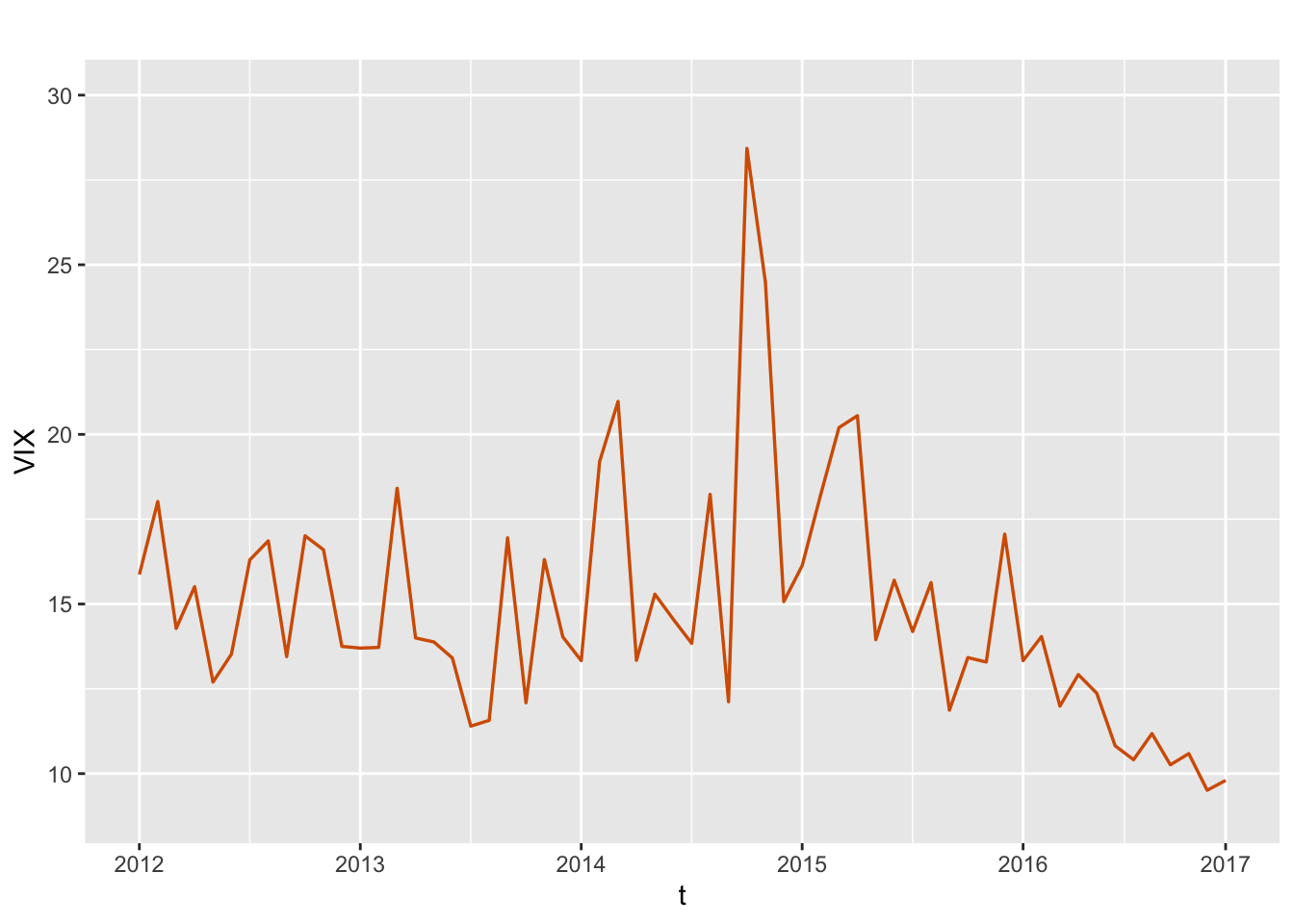
FIGURE 7.1: Monthly time series of VIX. The x-axis labels show the years for the data series.
Model G1
We first consider a model without regressors to explain the VIX time series. Specifically, assuming that \(\boldsymbol f'_t\) is \(1\), so that \(x_t\) denotes a random state, we write this model as
\[\begin{align} Y_t | \mu_t, \tau & \sim \text{Gamma}(\tau,\tau/\mu_t), \notag \\ \eta_t & = \log(\mu_t) = \alpha + x_t, \notag \\ x_t & = \phi x_{t-1} + w_t. \tag{7.4} \end{align}\] The formula and code for fitting the model are shown below. Figure 7.2 shows the observed and fitted VIX values from the fitted Model G1.
id.x <- 1:length(vix)
vix.data <- cbind.data.frame(vix, id.x)
formula.vix.G1 <-  vix ~  1 + f(id.x, model = "ar1")
model.vix.G1 <-  inla(
  formula.vix.G1,
  data = vix.data,
  family = "gamma",
  control.predictor = list(compute = TRUE),
  control.compute = list(
    dic = TRUE,
    waic = TRUE,
    cpo = TRUE,
    config = TRUE
  )
)
# summary(model.vix.G1)
format.inla.out(model.vix.G1$summary.fixed[,c(1:5)])
##   name      mean  sd    0.025q 0.5q 0.975q
## 1 Intercept 2.654 0.102 2.418  2.66 2.845
format.inla.out(model.vix.G1$summary.hyperpar[,(1:2)])
##   name                              mean   sd
## 1 Precision parameter for Gamma obs 47.137 11.941
## 2 Precision for id.x                42.556 24.436
## 3 Rho for id.x                       0.897  0.073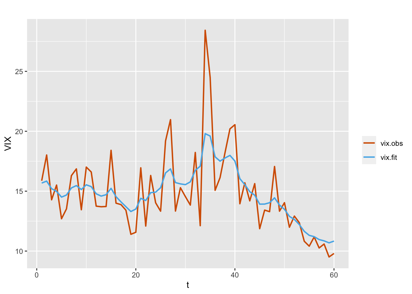
FIGURE 7.2: Observed (red) and fitted (blue) VIX values from the model without regressors (Model G1).
Note that the summary for the precision parameter \(\tau\) is given by “Precision parameter for Gamma obs” in model.vix.G1$summary.hyperpar. We can also obtain samples from the posterior distribution of \(\tau\) using inla.hyperpar.sample().
Model G2
As an alternative model, we can consider including another volatility index, VXN, as a regressor in the model. As noted by Aktekin, Polson, and Soyer (2020), “VXN is a measure of market expectations of 30-day volatility for the Nasdaq-100 market index, as implied by the price of near-term options on this index.” Figure 7.3 shows the overlay plot of the time series VIX and VXN, which suggests that the two indexes are positively correlated.
vxn <- index[, 2]
plot.df <- as_tibble(cbind.data.frame(
  time = id.x,
  vix.obs = vix.data$vix,
  vxn = vxn
))
multiline.plot(
  plot.df,
  title = "",
  xlab = "t",
  ylab = "VIX",
  line.size = 0.8,
  line.color = c("red", "black")
)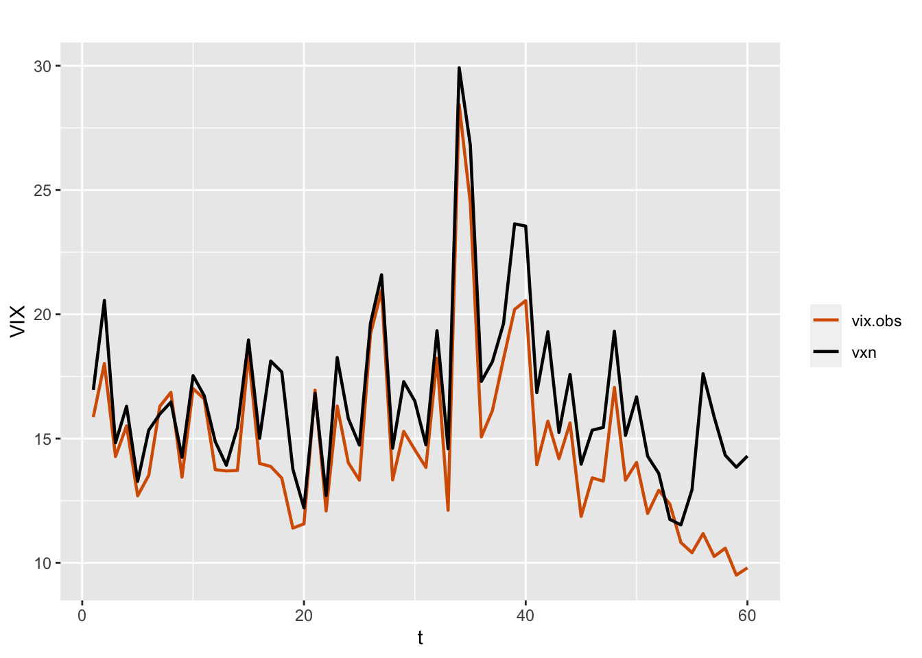
FIGURE 7.3: Monthly time series of VIX (red) and VXN (black).
Model G2 can be represented as
\[\begin{align} Y_t | \mu_t, \tau & \sim \text{Gamma}(\tau,\tau/\mu_t), \notag \\ \eta_t & =\alpha+\beta_t Z_t, \notag \\ \beta_t &= \phi \beta_{t-1} + w_t. \tag{7.5} \end{align}\] Here, \(\boldsymbol f_t\) is the VXN variable \(Z_t\). The results from this model are shown below, while observed and fitted VIX values are shown in Figure 7.4.
id.vxn <- id.x
formula.vix.G2 <- vix ~ 1 + f(id.vxn, vxn, model = "ar1")
model.vix.G2 <- inla(
  formula.vix.G2,
  data = vix.data,
  family = "gamma",
  control.predictor = list(compute = TRUE),
  control.compute = list(
    dic = TRUE,
    waic = TRUE,
    cpo = TRUE,
    config = TRUE
  )
)
# summary(model.vix.G2)
format.inla.out(model.vix.G2$summary.fixed[, c(1:5)])
## name mean sd 0.025q 0.5q 0.975q
## 1 Intercept 1.835 0.061 1.715 1.834 1.956format.inla.out(model.vix.G2$summary.hyperpar[, c(1:2)])## name mean sd
## 1 Precision parameter for Gamma obs 373.738 112.922
## 2 Precision for id.vxn 1651.985 932.790
## 3 Rho for id.vxn 0.994 0.004
FIGURE 7.4: Observed (red) and fitted (blue) VIX values from model with VXN as a dynamic regressor (Model G2).
Model G3
As a third example, we fit a model with a dynamic intercept term and a fixed effect corresponding to the regressor VXN:
\[\begin{align} Y_t | \mu_t, \tau & \sim \text{Gamma}(\tau,\tau/\mu_t), \notag \\ \eta_t & =\alpha+ \beta Z_t + x_t, \notag \\ x_t &= \phi x_{t-1} + w_t; \tag{7.6} \end{align}\] here, \(\boldsymbol f_t\) is \(1\). The code and the results from this model fit are given below.
formula.vix.G3 <-  vix ~ 1 + vxn + f(id.x, model = "ar1")
model.vix.G3 <- inla(
  formula.vix.G3,
  data = vix.data,
  family = "gamma",
  control.predictor = list(compute = TRUE),
  control.compute = list(
    dic = TRUE,
    waic = TRUE,
    cpo = TRUE,
    config = TRUE
  )
)
# summary(model.vix.G3)
format.inla.out(model.vix.G3$summary.fixed[, c(1:5)])
##   name      mean  sd    0.025q 0.5q  0.975q
## 1 Intercept 1.767 0.079 1.606  1.768 1.923
## 2 vxn       0.053 0.003 0.047  0.053 0.060
format.inla.out(model.vix.G3$summary.hyperpar[, c(1:2)])
##   name                              mean    sd
## 1 Precision parameter for Gamma obs 390.501 133.029
## 2 Precision for id.x                 97.510  41.649
## 3 Rho for id.x                        0.882   0.068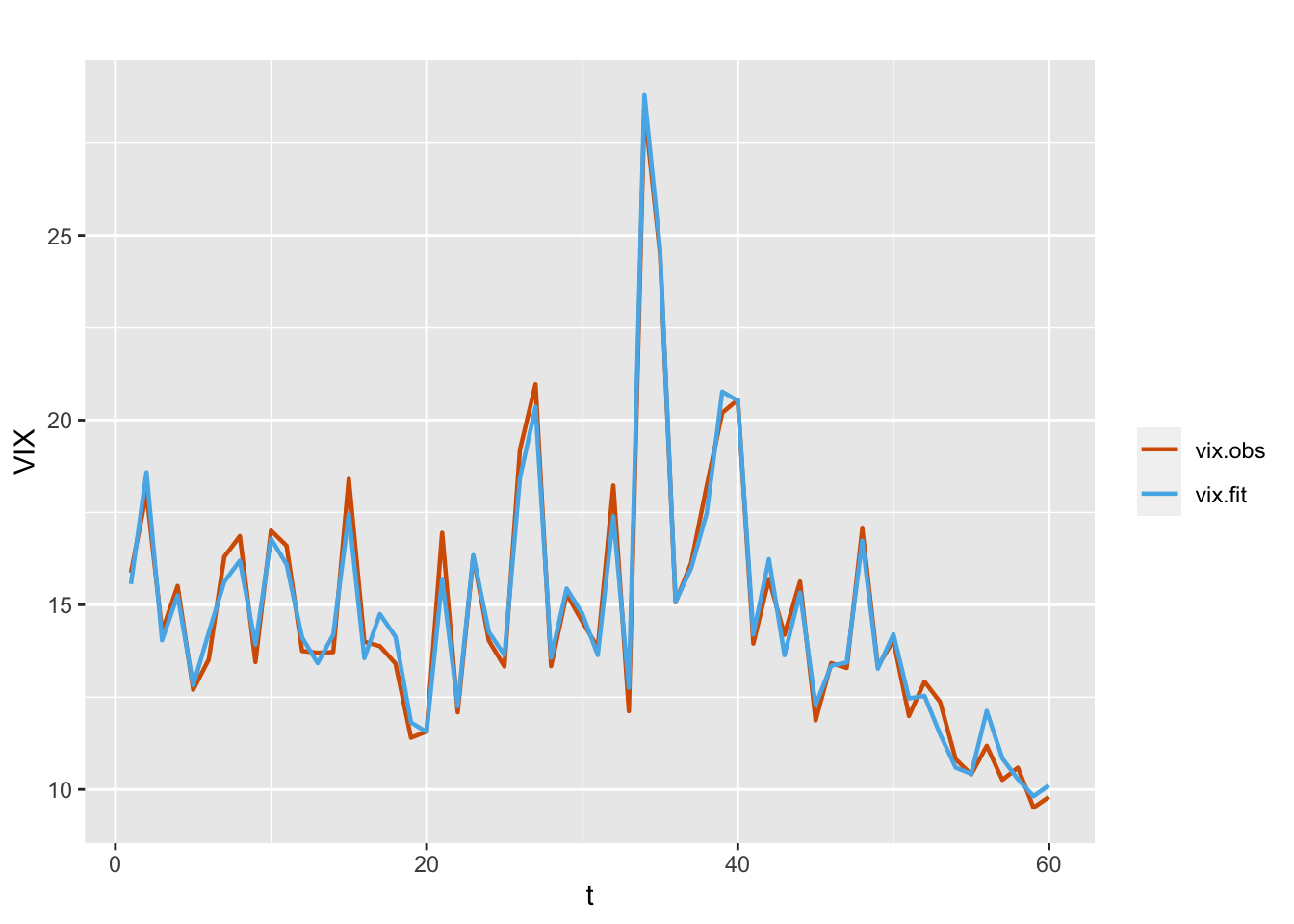
FIGURE 7.5: Observed (red) and fitted (blue) VIX values from a dynamic intercept and fixed VXN (Model G3).
In Table 7.1, we present a comparison of the three models. Based on the marginal likelihood as well as the DIC and WAIC, we see that Model G2 with a dynamic covariate effect does slightly better in terms of fit than Model G3, which has a dynamic intercept term but a static covariate effect.
| Model | DIC | WAIC | PsBF | Marginal likelihood |
|---|---|---|---|---|
| Model G1 | \(277.208\) | \(280.61\) | \(-142.295\) | \(-155.076\) |
| Model G2 | \(156.997\) | \(155.313\) | \(-81.417\) | \(-104.236\) |
| Model G3 | \(157.677\) | \(154.716\) | \(-82.49\) | \(-112.027\) |
As an alternative observation model for the VIX volatility index, we can consider a Weibull model, as discussed in the next section.
7.3 Weibull state space model
We can define a state space model for Weibull distributed observations.
Let \(Y_t \sim \text{Weibull}(\gamma_w, \lambda_t)\), where \(\gamma_w > 0\) is the static Weibull shape parameter and \(\lambda_t > 0\) is the dynamic scale parameter. R-INLA uses two different parameterizations for the Weibull density. The parameterization referred to as “variant 0” uses the following form of the Weibull density
\[\begin{align*} p(y_t|\gamma_w, \lambda_t)=\gamma_w\lambda_t y_t^{\gamma_w-1} e^{-\lambda_t y_t^{\gamma_w}}. \end{align*}\]
The alternative parameterization referred to as “variant 1” uses the density
\[\begin{align*} p(y_t|\gamma_w, \lambda_t)=\gamma_w\lambda_t^{\gamma_w} y_t^{\gamma_w-1} e^{-(\lambda_t y_t)^{\gamma_w}}. \end{align*}\]
For both parameterizations, the linear predictor is defined as
\[\begin{align} \eta_t=\log(\lambda_t) &= \alpha + \boldsymbol f'_t \boldsymbol x_t, \mbox{ with}, \notag \\ \boldsymbol x_t &= \boldsymbol G \boldsymbol x_{t-1}+ \boldsymbol w_t, \tag{7.7} \end{align}\] where \(\boldsymbol x_t\) is an \(h\)-dimensional state vector, \(\boldsymbol f_t\) is a \(h\times 1\) covariate vector, \(\boldsymbol G\) is an \(h\times h\) transition matrix, and \(\boldsymbol w_t \sim N(\boldsymbol 0,\boldsymbol W)\).
Model W1
We first fit a model with a dynamic intercept, but without any regressors. The model has the same structure as Model G1. The observed and fitted VIX values are shown in Figure 7.6. The choice of model variant is given in control.family.
formula.vix.W1 <- vix ~ 1 + f(id.x, model = "ar1")
model.vix.W1 <- inla(
  formula.vix.W1,
  data = vix.data,
  family = "weibull",
  control.family = list(variant = 0),
  control.predictor = list(compute = TRUE, link = 1),
  control.compute = list(
    dic = TRUE,
    waic = TRUE,
    cpo = TRUE,
    config = TRUE
  )
)
# summary(model.vix.W1)
format.inla.out(model.vix.W1$summary.fixed[, c(1:5)])
##   name      mean   sd    0.025q 0.5q   0.975q
## 1 Intercept -22.65 2.723 -30.6  -21.88 -19.2
format.inla.out(model.vix.W1$summary.hyperpar[, c(1:2)])
##   name                        mean  sd
## 1 alpha parameter for weibull 9.182 1.039
## 2 Precision for id.x          0.282 0.108
## 3 Rho for id.x                0.849 0.088
Note that \(\gamma_w\) in our notation corresponds to “alpha parameter for Weibull” in the inla() output.
For obtaining fitted values, the standard procedure of using model.vix.W1$summary.fitted.values$mean will lead to incorrect fits. The suggested procedure to obtain fits for the Weibull family is to use inla.posterior.sample() as shown below. Discussion on the function fun.pred() follows after the code.
post.sample.W1 <-
  inla.posterior.sample(n = 1000, model.vix.W1, seed = 123457)
fun.pred <- function(x) {
  return(gamma(1 + 1 / x$hyperpar[1]) /
           (exp(x$latent[1:n]) ^ (1 / x$hyperpar[1])))
}
fits <- post.sample.W1 %>%
  sapply(function(x)
    fun.pred(x))
fit.vix.W1 <- rowMeans(fits)
plot.df <- as_tibble(cbind.data.frame(
  time = id.x,
  vix.obs = vix.data$vix,
  vix.fit = fit.vix.W1
))
multiline.plot(
  plot.df,
  title = "",
  xlab = "t",
  ylab = "VIX",
  line.size = 0.8,
  line.color = c("red", "blue")
)
FIGURE 7.6: Observed (red) and fitted (blue) values from the model without regressors (Model W1).
Since we have used the parameterization variant=0 in Model W1, the fitted values are obtained using the transformation
\[\begin{align*} E(y_t|\gamma_w, \lambda_t)=\lambda_t^{-1/\gamma_w}\Gamma(1+1/\gamma_w). \end{align*}\]
If the parameterization “variant=1” is used, similar results can be obtained for fitted values via the transformation
\[\begin{align*} E(y_t|\gamma_w, \lambda_t)=\lambda_t^{-1}\Gamma(1+1/\gamma_w). \end{align*}\]
Model W2
The Weibull analog of Model G2 (model with VXN as regressor with a dynamic coefficient) is shown below. For illustrative purposes, we ran this model using variant=1.
id.vxn <- 1:length(vxn)
vix.data <- cbind.data.frame(vix.data, id.vxn, vxn)
formula.vix.W2 = vix ~ 1 + f(id.vxn,vxn, model = "ar1")
model.vix.W2 = inla(
  formula.vix.W2,
  data = vix.data,
  family = "weibull",
  control.family = list(variant = 1),
  control.predictor = list(compute = TRUE, link = 1),
  control.compute = list(
    dic = TRUE,
    waic = TRUE,
    cpo = TRUE,
    config = TRUE
  )
)
# summary(model.vix.W2)
format.inla.out(model.vix.W2$summary.fixed[, c(1:5)])
##   name      mean   sd    0.025q 0.5q   0.975q
## 1 Intercept -1.833 0.061 -1.956 -1.832 -1.714
format.inla.out(model.vix.W2$summary.hyperpar[, c(1:2)])
##   name                        mean     sd
## 1 alpha parameter for weibull   25.050   3.866
## 2 Precision for id.vxn        1533.827 891.956
## 3 Rho for id.vxn                 0.992   0.006
7.3.1 Forecasting from Weibull models
As in the computation of fitted values, evaluation of forecasts from the Weibull state space model requires use of the mean of the Weibull model with scale parameter \(\lambda_t\) and shape parameter \(\gamma_w\). For both parameterizations, INLA uses the linear predictor \(\eta_t=\log(\lambda_t)\).
For example, in Model W1 we have
\[\begin{align} Y_t | \lambda_t, \gamma_w & \sim \text{Weibull}(\lambda_t, \gamma_w), \notag \\ \eta_t & = \log(\lambda_t) = \alpha + x_t, \notag \\ x_t & = \phi x_{t-1} + w_t. \tag{7.8} \end{align}\] It follows from the above that
\[\begin{align*} x_t|x_{t-1},\phi,\sigma^2_w\sim N(\phi x_{t-1},\sigma^2_w). \end{align*}\]
After observing data from \(n\) periods, i.e., \(\boldsymbol y^{n}=(y_1,\ldots,y_n)\), we have posterior distributions of \(\alpha,\,\sigma^2_w,\,\phi\) and \(\,x_n\). To predict the next observation \(y_{n+1}\), we need the posterior mean of \(y_{n+1}\) given \(\boldsymbol y^{n}\), i.e.,
\[\begin{align*} E(y_{n+1}|\boldsymbol y^{n}) =E\Bigl[E(y_{n+1}|\alpha,\,\gamma_w,\sigma^2_w,\,\phi, x_{n+1})\Bigr], \end{align*}\] where the outside expectation is taken with respect to the joint posterior distribution of \(\alpha,\,\gamma_w,\sigma^2_w,\,\phi\) and \(x_{n+1}\), and
\[\begin{align*} E(y_{n+1}|\alpha,\,\sigma^2_w,\,\phi,\text{ }x_{n+1}) = \begin{cases} \lambda^{-1/\gamma_w}_{n+1}\,\Gamma(1+1/\gamma_w)\text{, for variant}=0&\\ \lambda^{-1}_{n+1}\,\,\,\,\,\Gamma(1+1/\gamma_w)\text{, for variant}=1.& \end{cases} \end{align*}\]
We can evaluate \(E(y_{n+1}|\boldsymbol y^{n})\) by a Monte Carlo average based on \(M\) samples from the posterior distribution of \(\alpha,\,\gamma_w,\sigma^2_w,\,\phi\), and \(x_{n+1}\), for large \(M\). Specifically, for each realization of \((x_n,\phi,\sigma^2_w)\), we draw samples of \(x_{n+1}\) from \(N(\phi x_n,\sigma^2_w)\), and for each realization of \((x_{n+1},\alpha)\), we obtain samples of \(\eta_{n+1}=\alpha+x_{n+1}\) and \(\lambda_{n+1}=e^{\eta_{n+1}}\). Finally, for each realization of \((\lambda_{n+1},\gamma_w)\) we evaluate \(E(y_{n+1}|\alpha,\,\sigma^2_w,\,\phi, x_{n+1})\), and use the Monte Carlo average as our prediction. Similarly, predictions for \(y_{n+2},\ldots,y_{n+L}\) will require use of the conditional distribution \(x_t|x_{t-1},\phi,\sigma^2_w\) for \(t=n+2,\ldots,n+L\) in a sequential manner. We show the code for forecasting under Model W1.
mean <-
  post.sample.W1[[1]]$hyperpar['Rho for id.x'] *
  post.sample.W1[[1]]$latent[2 * n]
sigma2.w <- 1 / post.sample.W1[[1]]$hyperpar['Precision for id.x']
x.np1 <- rnorm(500, mean = mean, sd = sqrt(sigma2.w))
eta.np1 <- c(tail(post.sample.W1[[1]]$latent, 1)) + x.np1
lambda.np1 <- exp(eta.np1)
gamma.w <-
  post.sample.W1[[1]]$hyperpar['alpha parameter for weibull']
y.np1 <- gamma(1 + 1 / gamma.w) /
  (lambda.np1 ^ (1 / gamma.w))
mean(y.np1)
## [1] 12.17
7.4 Beta state space model
Let \(Y_t \sim \text{Beta}(\tau\gamma_t,\tau(1-\gamma_t))\), where \(\,0<\gamma_t<1\). Note that \(E(Y_t|\gamma_t)=\gamma_t\), and \(Var(Y_t|\gamma_t,\tau)=\gamma_t(1-\gamma_t)/(\tau+1)\), implying that \(\tau\) is a precision parameter. We assume that
\[\begin{align} \eta_t &=\log(\gamma_t/(1-\gamma_t))= \alpha+ \boldsymbol f'_t \boldsymbol x_t, \notag \\ \boldsymbol x_t &= \boldsymbol G \boldsymbol x_{t-1}+ \boldsymbol w_t, \end{align}\] where \(\alpha\) is an intercept term, \(\boldsymbol x_t\) is an \(h\)-dimensional state vector, \(\boldsymbol f_t\) is an \(h\)-dimensional covariate vector, \(\boldsymbol G\) is an \(h\times h\) transition matrix, and \(\boldsymbol w_t \sim N(\boldsymbol 0,\boldsymbol W)\).
7.4.1 Example: Crest market share
We consider weekly market share data for Crest used by Wichern and Jones (1977) for intervention analysis. Historically, Crest toothpaste was introduced nationally in 1956 when Colgate was enjoying a significant portion of the market share. This dominance of Colgate continued until 1960, and Crest’s market share during this period was relatively stable, but in August 1, 1960, the American Dental Association (ADA) endorsed Crest as an “important aid in any program of dental hygiene.” In what follows, we first show a time series plot of Crest’s market share in Figure 7.7, where the ADA endorsement date of August 1, 1960, is presented by a vertical dashed line at \(t=135\). As shown in this plot, there is a clear jump in Crest’s market following the endorsement, suggesting nonstationarity in the data.
mshare <- read.csv("TPASTE.csv", header = TRUE)
crestms <- mshare[, 1]
tsline(crestms,
        ylab = "market share",
        xlab = "week",
       line.color = "red",
       line.size = 0.6) +
  geom_vline(xintercept = 135, linetype="dashed", color = "black")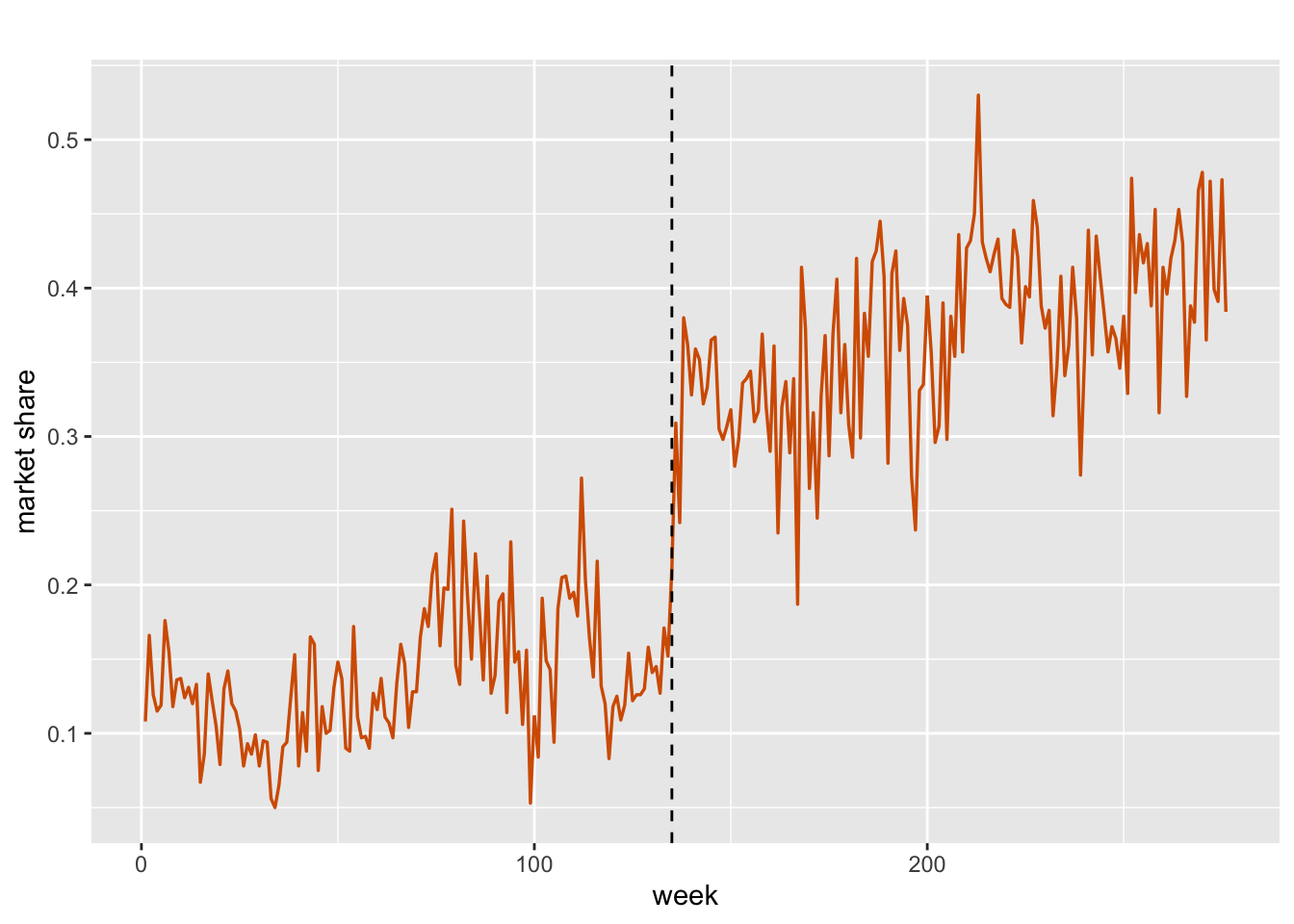
FIGURE 7.7: Weekly market share of Crest toothpaste. The vertical line (black) denotes Aug 1, 1960.
# abline(v = 135, col = "blue", lty = 2)As in the previous section, if we do not have any regressors, then \(\eta_t=\alpha+x_t\) will be a scalar, and the state equation will reduce to
\[\begin{align} x_t= G x_{t-1}+ w_t, \end{align}\] where \(G\) is a scalar and and \(w_t\) is a univariate white noise process.
Model B1
We first consider the model without any regressors, i.e.,
\[\begin{align} \eta_t & =\alpha+x_t, \notag\\ x_t &= \phi x_{t-1} + w_t. \tag{7.9} \end{align}\] We estimate the model using the code below and show the plot of fitted versus the observed values in Figure 7.8.
id.x <- 1:length(crestms)
crest.data <- cbind.data.frame(mshare, id.x)
formula.crest.B1 = crestms ~ 1 + f(id.x, model = "ar1")
model.crest.B1 = inla(
  formula.crest.B1,
  data = crest.data,
  family = "beta",
  scale = 1,
  control.predictor = list(compute = TRUE),
  control.compute = list(
    dic = TRUE,
    waic = TRUE,
    cpo = TRUE,
    config = TRUE
  )
)
# summary(model.crest.B1)
format.inla.out(model.crest.B1$summary.fixed[, c(1:5)])
##   name      mean   sd   0.025q 0.5q   0.975q
## 1 Intercept -1.159 0.46 -2.106 -1.162 -0.191
format.inla.out(model.crest.B1$summary.hyperpar[, c(1:2)])
##   name                             mean   sd
## 1 precision parameter for beta obs 114.87 11.897
## 2 Precision for id.x                 2.56  1.236
## 3 Rho for id.x                       0.99  0.005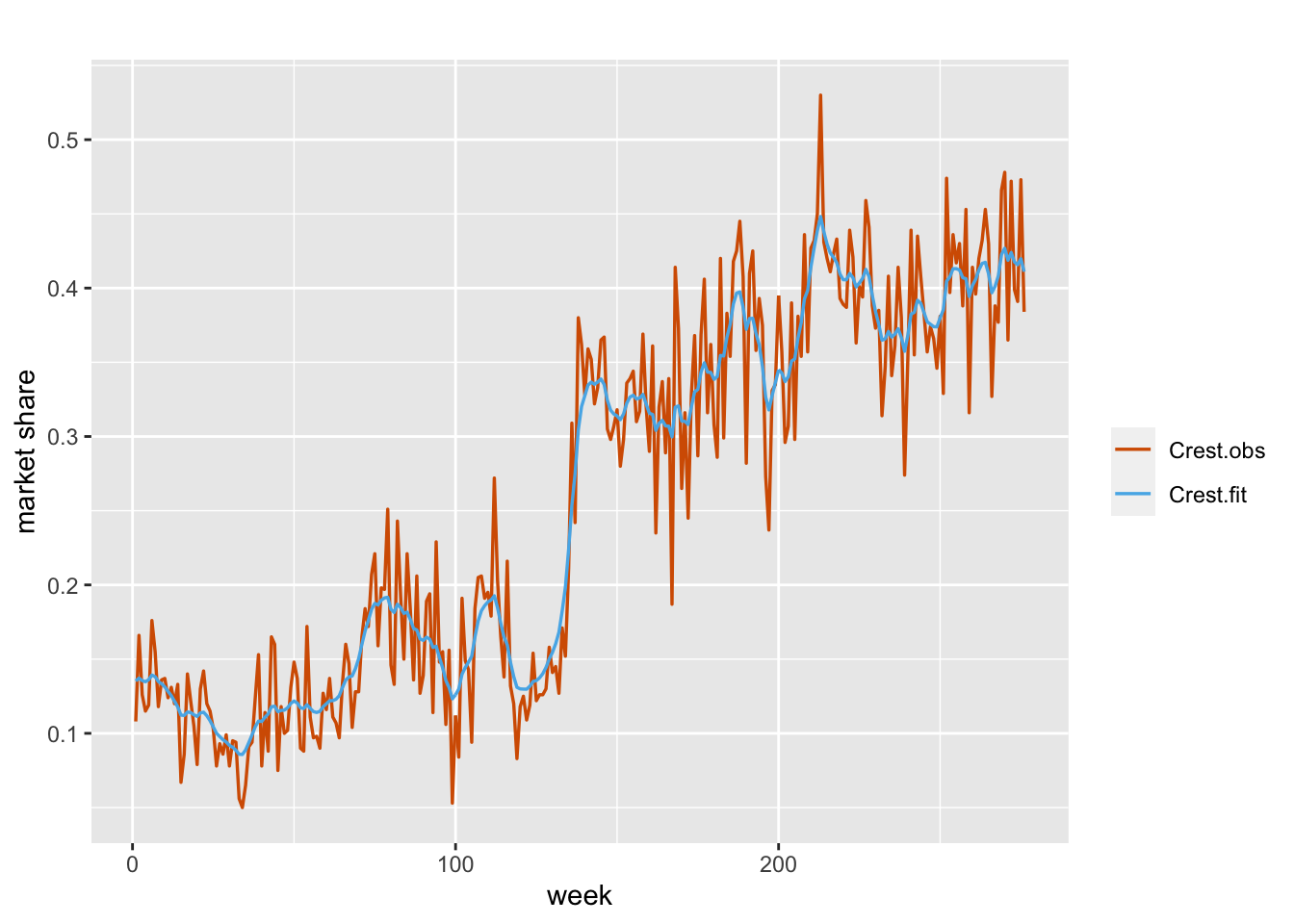
FIGURE 7.8: Observed (red) and fitted (blue) values from Model B1 for the Crest data.
Model B2
Next, we bring in three regressors, the market share for Colgate (colgms), unit price for Crest (crestpr), and unit price for Colgate (colgpr). We treat them all as fixed, but include a dynamic intercept term, i.e.,
\[\begin{align} \eta_t & =\alpha+\beta_1 Z_{1t}+\beta_2 Z_{2t}+\beta_3 Z_{3t}+x_t, \notag \\ x_t &= \phi x_{t-1} + w_t. \tag{7.10} \end{align}\]
The plot of the actual versus fitted series is shown in Figure 7.9.
colgms <- mshare[, 2]
crestpr <- mshare[, 3]
colgpr <- mshare[, 4]
formula.crest.B2 <-
  crestms ~ 1 + colgms + crestpr + colgpr + f(id.x, model = "ar1")
model.crest.B2 <- inla(
  formula.crest.B2,
  data = crest.data,
  family = "beta",
  scale = 1,
  control.predictor = list(compute = TRUE),
  control.compute = list(
    dic = TRUE,
    waic = TRUE,
    cpo = TRUE,
    config = TRUE
  )
)
# summary(model.crest.B2)
format.inla.out(model.crest.B2$summary.fixed[, c(1:5)])
##   name      mean   sd    0.025q 0.5q   0.975q
## 1 Intercept  2.371 0.779  0.818  2.378  3.881
## 2 colgms    -2.593 0.315 -3.212 -2.593 -1.976
## 3 crestpr   -0.887 0.241 -1.360 -0.887 -0.413
## 4 colgpr    -0.515 0.286 -1.077 -0.516  0.047
format.inla.out(model.crest.B2$summary.hyperpar[, c(1:2)])
##   name                             mean    sd
## 1 precision parameter for beta obs 135.576 13.737
## 2 Precision for id.x                 6.954  3.184
## 3 Rho for id.x                       0.985  0.007
The signs for the coefficients of colgms and crestpr are negative, as expected. While the sign of colgpr being negative is not as easy to explain, we note that this coefficient is not significantly different than zero.
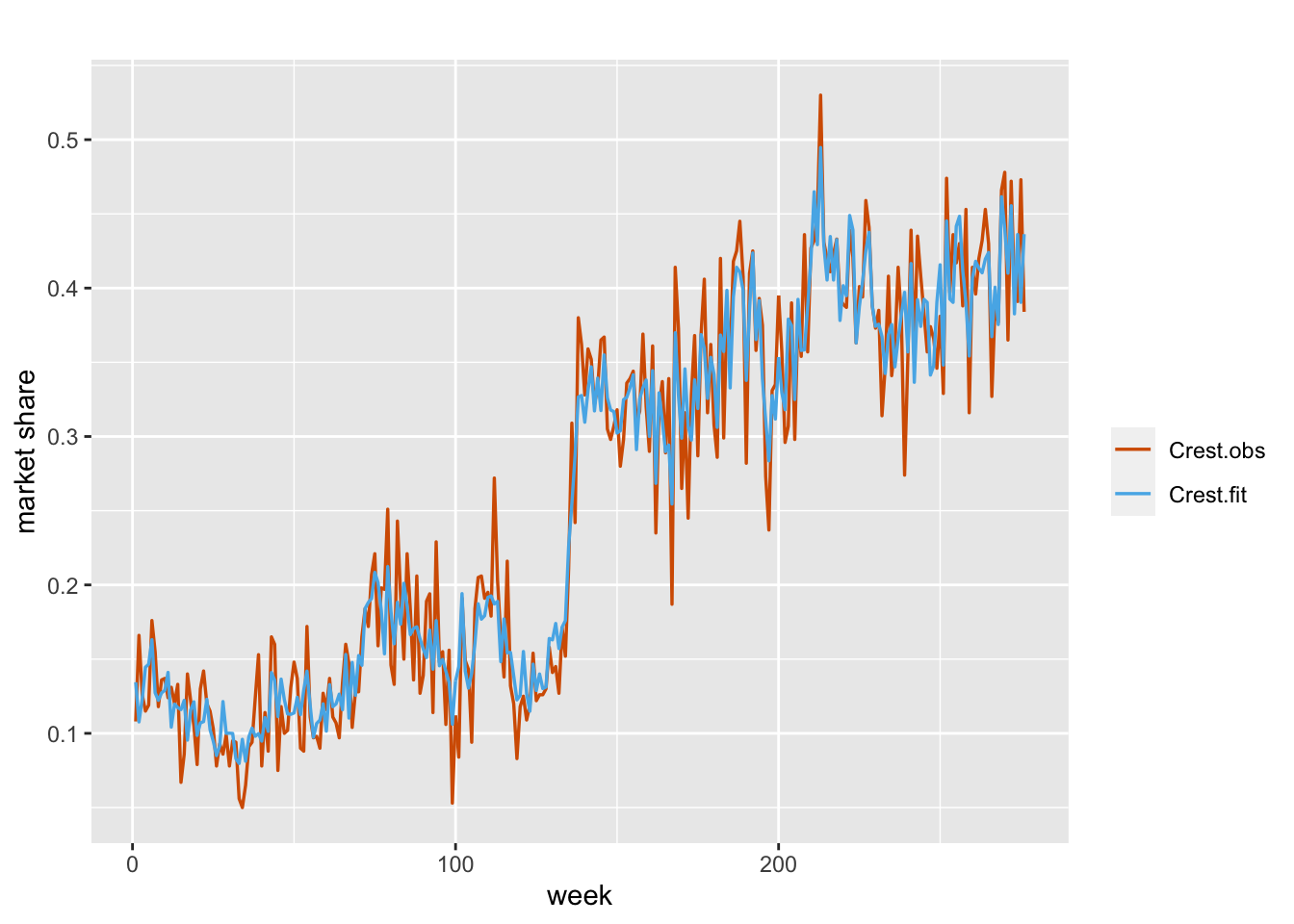
FIGURE 7.9: Observed (red) and fitted (blue) values from Model B2 for the Crest data.
Model B3
Our third model will have dynamic coefficients for all three covariates. Specifically, we have
\[\begin{align} \eta_t & =\alpha+\beta_{1t} Z_{1t}+\beta_{2t} Z_{2t}+\beta_{3t} Z_{3t}, \notag \\ \beta_{1t} &= \phi_1 \beta_{1,t-1} + w_{1t}, \notag \\ \beta_{2t} &= \phi_2 \beta_{2,t-1} + w_{2t}, \notag\\ \beta_{3t} &= \phi_3 \beta_{3,t-1} + w_{3t}. \tag{7.11} \end{align}\] We show a plot of actual versus fitted observations in Figure 7.10.
id.colgms <- id.crestpr <- id.colgpr <- 1:length(crestms)
formula.crest.B3 <-
  crestms ~ 1 + f(id.colgms, colgms, model = "ar1") +
  f(id.crestpr, crestpr, model = "ar1") +
  f(id.colgpr, colgpr, model = "ar1")
model.crest.B3 <- inla(
  formula.crest.B3,
  data = crest.data,
  family = "beta",
  scale = 1,
  control.predictor = list(compute = TRUE),
  control.compute = list(
    dic = TRUE,
    waic = TRUE,
    cpo = TRUE,
    config = TRUE
  )
)
# summary(model.crest.B3)
format.inla.out(model.crest.B3$summary.fixed[, c(1:5)])
##   name      mean  sd    0.025q 0.5q  0.975q
## 1 Intercept 0.138 0.527 -0.837 0.129 1.191
format.inla.out(model.crest.B3$summary.hyperpar[, c(1:2)])
##   name                             mean      sd
## 1 precision parameter for beta obs   116.106    12.072
## 2 Precision for id.colgms          22971.649 23826.284
## 3 Rho for id.colgms                    0.031     0.674
## 4 Precision for id.crestpr             5.214     3.632
## 5 Rho for id.crestpr                   0.995     0.003
## 6 Precision for id.colgpr          22648.905 21768.024
## 7 Rho for id.colgpr                    0.047     0.674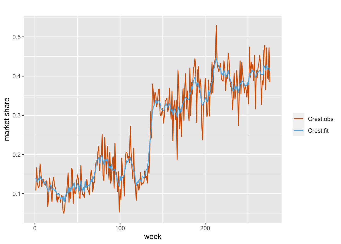
FIGURE 7.10: Observed (red) and fitted (blue) values from Model B3 for the Crest data.
Model B4
We can also try fitting a standard static beta regression model as a benchmark, i.e.,
\[\begin{align} \eta_t & =\alpha+\beta_1 Z_{1t}+\beta_2 Z_{2t}+\beta_3 Z_{3t}. \tag{7.12} \end{align}\] The fit of the model is shown in Figure 7.11.
formula.crest.B4 <- crestms ~ 1 + colgms + crestpr + colgpr
model.crest.B4 <- inla(
  formula.crest.B4,
  data = crest.data,
  family = "beta",
  scale = 1,
  control.predictor = list(compute = TRUE),
  control.compute = list(
    dic = TRUE,
    waic = TRUE,
    cpo = TRUE,
    config = TRUE
  )
)
# summary(model.crest.B4)
format.inla.out(model.crest.B4$summary.fixed[, c(1:5)])
##   name      mean   sd    0.025q 0.5q   0.975q
## 1 Intercept  6.285 0.395  5.509  6.286  7.059
## 2 colgms    -4.196 0.411 -5.004 -4.196 -3.390
## 3 crestpr   -2.649 0.245 -3.130 -2.649 -2.168
## 4 colgpr    -0.485 0.252 -0.979 -0.485  0.009
format.inla.out(model.crest.B4$summary.hyperpar[, c(1:2)])
##   name                             mean  sd
## 1 precision parameter for beta obs 44.45 3.763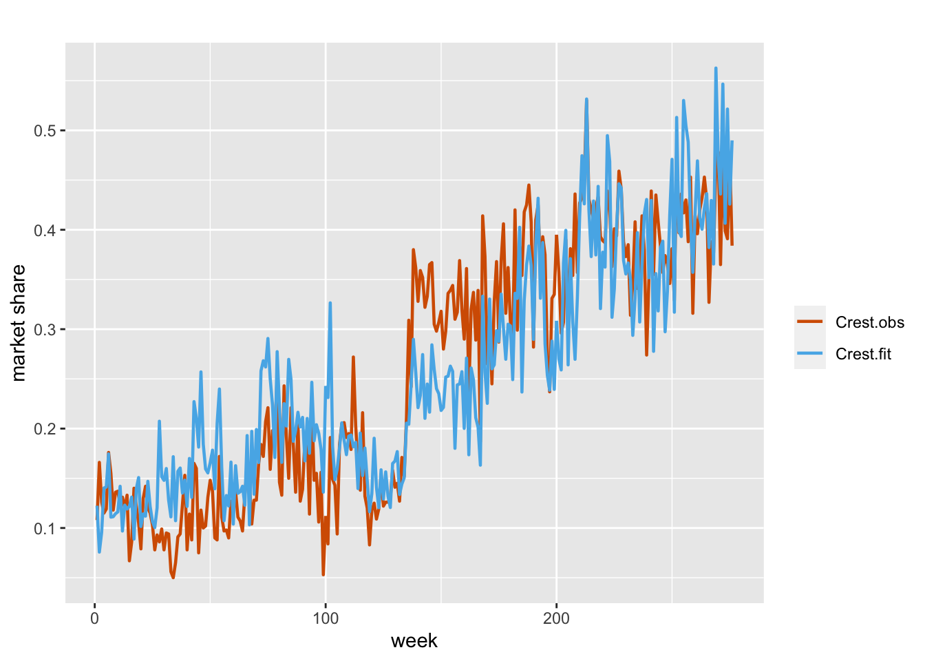
FIGURE 7.11: Observed and fitted values from Model B4 for the Crest data.
We present a comparison of all the models in Table 7.2. Note that among the four models, Model B2, where we have static regression coefficients and a dynamic intercept, gives the best fit.
| Model | DIC | WAIC | PsBF | Marginal Likelihood |
|---|---|---|---|---|
| Model B1 | \(-994.35\) | \(-996.223\) | \(495.744\) | \(446.508\) |
| Model B2 | \(-1052.07\) | \(-1054.711\) | \(525.875\) | \(469.797\) |
| Model B3 | \(-998.985\) | \(-1001.029\) | \(498.292\) | \(449.91\) |
| Model B4 | \(-771.608\) | \(-772.073\) | \(386.034\) | \(368.948\) |